Quickstart Guide
This guide introduces the core concept and components of outset plots, then covers how to create them using the outset.OutsetGrid interface.
The outset.OutsetGrid class provides a FacetGrid-like interface to arrange magnifications of plotted data on an axes grid. With this API, magnification frame positioning is automatically determined based on the structure of dataframe content.
The FacetGrid class also supports manual specification of magnified areas, covered subsequently. This interface broadcasts identical plot content over all grid axes then sets individual axes’ data limits to create magnification panels.
The final sections of the guide cover detail aspect ratio management, layout control, and styling — including how to use outset.inset_outsets to transform an OutsetGrid to render magnification plots as inset axes over the main plot, instead of abreast in a grid with the main plot. In addition to outset.OutsetGrid, lower-level outset.marqueeplot and outset.draw_marquee APIs can be used directly for more bespoke applications.
Table of Contents
[1]:
from matplotlib import cbook as mpl_cbook
from matplotlib import pyplot as plt
import numpy as np
import outset as otst
from outset import mark as otst_mark
from outset import patched as otst_patched
from outset import tweak as otst_tweak
from outset import util as otst_util
import pandas as pd
import seaborn as sns
Some imports and setup.
Taxonomy: Marquees, Outsets, and Insets
[2]:
# --- Data Preparation ---
# Create a DataFrame with sample data defining the extent of marquee elements
plot_data = pd.DataFrame(
    {
        "x_values": [0, 2, 5.8, 6],
        "y_values": [1, 4, 8, 9],
        "group": ["group1", "group1", "group2", "group2"],
    }
)

# --- Plot Initialization ---
# Initialize an OutsetGrid object for creating plots with grouped data.
outset_grid = otst.OutsetGrid(  # API is a la FacetGrid
    data=plot_data,
    x="x_values",
    y="y_values",
    col="group",
    hue="group",
    marqueeplot_kws={"mark_glyph_kws": {"markersize": 15}},
)

# --- Rendering ---
# Draw marquee elements.
outset_grid.marqueeplot()

# --- Annotations ---
# Label plot elements.

# Annotate a callout mark.
outset_grid.source_axes.annotate(
    "callout mark",
    xy=(3, 4.5),
    xytext=(3.5, 3.5),
    horizontalalignment="left",
    arrowprops=dict(arrowstyle="->", lw=1),
)

# Annotate a callout leader.
outset_grid.source_axes.annotate(
    "callout leader",
    xy=(2.5, 3.5),
    xytext=(3.5, 2.5),
    horizontalalignment="left",
    arrowprops=dict(arrowstyle="->", lw=1),
)

# Annotate the frame.
outset_grid.source_axes.annotate(
    "frame",
    xy=(1, 2),
    xytext=(1, 2),
    horizontalalignment="center",
)

# Annotate the marquee.
outset_grid.source_axes.annotate(
    "marquee",
    xy=(1.5, 6),
    xytext=(1.5, 6.5),
    ha="center",
    va="bottom",
    arrowprops=dict(
        arrowstyle="-[, widthB=4.0, lengthB=1.0", lw=2.0, color="k"
    ),
)

# --- Finalization ---
# Customize titles for the source and outset axes.
outset_grid.broadcast_source(lambda ax: ax.set_title("source axes"))
outset_grid.broadcast_outset(lambda ax: ax.set_title("outset axes"))

pass  # sponge up last return value, if any
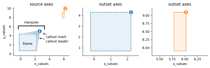
The outset library creates multi-scale data visualizations that composite a “source” plot with magnified subsection views. These excerpted plot elements are termed as “outsets.”
The zoom relationships between a source plot and accompanying outsets is indicated by “marquee” frame annotations. A marquee is composed of (1) a bounding frame and (2) a callout, containing (i) an angled leader that tapers to (ii) an identifying mark.
The figure-level outset.OutsetGrid wrangles orchesration of these figure elements over an axis grid, composed of the source plot beside outset magnified panels. Magnified regions, as well as figure styling and layout, are specified via the OutsetGrid initializer. The OutsetGrid.map_dataframe and OutsetGrid.broadcast methods facilitate population of axes grid content. The OutsetGrid.marqueeplot method, usually called last, dispatches rendering of marquee annotations. The next
sections will cover how to initialize and populate OutsetGrid plots in detail.
[3]:
# ... continue working on outset_grid object from previous frame

# --- Inset and Outset Creation ---
# Rearrange outset axes as insets onto the source plots
otst.inset_outsets(outset_grid, insets="NW")

# --- Additional Annotations ---
# Further annotate to label the inset and outset axes.

# Annotate the inset and outset axes with an arrow pointing to them.
outset_grid.source_axes.annotate(
    "inset\noutset\naxes",
    xy=(3.5, 8.7),
    xytext=(3.9, 8.7),
    clip_on=False,
    ha="left",
    va="center",
    arrowprops=dict(
        arrowstyle="-[, widthB=1.5, lengthB=0.5", lw=2.0, color="k"
    ),
)

# Add an arrow pointing upwards without text to indicate a specific area.
outset_grid.source_axes.annotate(
    "",
    xy=(2.5, 10.2),
    xytext=(2.5, 10.21),
    clip_on=False,
    ha="center",
    va="bottom",
    arrowprops=dict(arrowstyle="-[, widthB=10, lengthB=0.5", lw=2.0, color="k"),
    annotation_clip=False,
)

# --- Display ---
# Render and display the figure with all the elements.
# Must call explicitly to draw a second time after render in previous frame.
display(outset_grid.figure)

pass  # sponge up last return value, if any
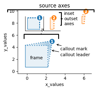
If desired, outset axes can be transformed into insets over the source axes by running an OutsetGrid through the outset.inset_outsets function.
[4]:
# --- Data Preparation ---
# Create a DataFrame with sample data defining the extent of marquee elements
data = pd.DataFrame(
    {
        "x": [0, 0.2, 2.3, 1.8, 0.5, 2, 5.8, 5.87, 5.95, 6, 6],
        "y": [1, 2, 2.9, 3, 1.5, 4, 8, 8.2, 8.6, 9, 10],
        "outset": [
            "group1",
            "group1",
            "group1",
            "group1",
            "group1",
            "group1",
            "group2",
            "group2",
            "group2",
            "group2",
            "group2",
        ],
    }
)

# --- Plot Initialization ---
# Initialize an OutsetGrid object for creating plots with grouped data.
outset_grid = otst.OutsetGrid(
    data=data,
    x="x",
    y="y",
    col="outset",
    hue="outset",
    marqueeplot_kws={"mark_glyph_kws": {"markersize": 15}},
)

# --- Mapping Data ---
# Map filled then outline KDE plot (filled) across all axes
outset_grid.map_dataframe(
    sns.kdeplot,
    x="x",
    y="y",
    alpha=0.2,
    levels=2,
    legend=False,
    fill=True,
    thresh=0.01,
)
outset_grid.map_dataframe(
    sns.kdeplot,
    x="x",
    y="y",
    levels=2,
    legend=False,
    thresh=0.01,
)

# Scatter data on all axes.
outset_grid.map_dataframe(sns.scatterplot, x="x", y="y", legend=False)

# --- Finalization ---
# Set titles for the source and outset axes.
outset_grid.broadcast_source(lambda ax: ax.set_title("source axes"))
outset_grid.broadcast_outset(lambda ax: ax.set_title("outset axes"))

# Add a legend and fix any introduced skew
outset_grid.add_legend()
outset_grid.equalize_aspect()

# --- Annotations ---
# Annotate to indicate a data group on the plot.
outset_grid.source_axes.annotate(
    "data group",
    xy=(1, 6),
    xytext=(1, 6.5),
    ha="center",
    va="bottom",
    arrowprops=dict(
        arrowstyle="-[, widthB=5.0, lengthB=1.0", lw=2.0, color="k"
    ),
)

pass  # sponge up last return value, if any
No artists with labels found to put in legend. Note that artists whose label start with an underscore are ignored when legend() is called with no argument.
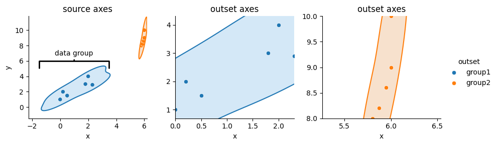
Marquee annotations are optional, and can eschewed by simply not calling OutsetGrid.marqueeplot.
Inferred Zoom Areas
The outset.OutsetGrid class closely tracks the design and API conventions of seaborn.FacetGrid. You can think of an OutsetGrid as a FacetGrid with an unfaceted (i.e., all data) plot tacked on the front and some additional mechanisms for control of axes data limits.
[5]:
# --- Plot Initialization ---
# Initialize an OutsetGrid object for creating a series of scatter plots.
# The plots will be based on the 'table' and 'depth' features, categorized by
# the 'cut' of the diamonds.
og = otst.OutsetGrid(
    data=sns.load_dataset("diamonds").dropna(),
    aspect=1.5,  # Set aspect ratio
    x="table",
    y="depth",
    col="cut",
    col_order=["Premium"],  # Focus on 'Premium' cut diamonds only
    marqueeplot_kws={
        "mark_glyph": otst_mark.MarkRomanBadges,  # Use Roman badge markers
        "leader_stretch": 0.2,
        "leader_stretch_unit": "inches",
        "leader_tweak": otst_tweak.TweakReflect(horizontal=True),
    },
)

# --- Draw Data ---
# Map scatter plot over all axes.
og.map_dataframe(
    otst_patched.scatterplot,
    x="table",
    y="depth",
    legend=False,  # No individual legend for plots
    zorder=-2,
    color="gray",
    s=otst_util.SplitKwarg(  # pass different args to source vs. outset axes
        source=10,  # Size for source markers
        outset=10,  # Size for outset markers
    ),
)

# --- Finalization ---
# Set a title and add a legend
og.source_axes.set_title("cut = All")

# Render marquee elements
og.marqueeplot()

pass  # sponge up last return value, if any
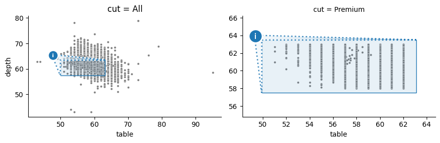
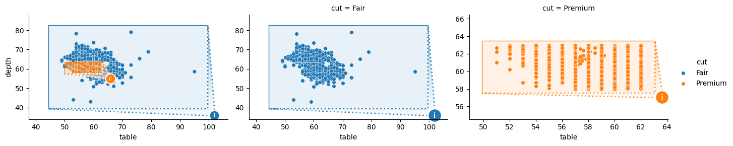
Here, OutsetGrid(col="cut", col_order=["Premium"]) have been specified. This indicates that the dataframe subset where df["cut"] == "Premium" should be plotted as an outset. Then, OutsetGrid.map_dataframe(sns.scatterplot) is called to render data — all data on the source plot and “Premium” cut data on the outset. Finally, OutsetGrid.marqueeplot adds marquee annotations and finalizes axes data limits.
[6]:
# --- Plot Initialization ---
# Initialize an OutsetGrid object to create plots with grouped data.
# The plots will be based on 'table' and 'depth' features, categorized by 'cut'.
outset_grid = otst.OutsetGrid(
    data=sns.load_dataset("diamonds").dropna(),
    aspect=1.5,
    x="table",
    y="depth",
    col="cut",
    col_order=["Fair", "Premium"],  # Focus on 'Fair' and 'Premium' cuts only.
    hue="cut",
    hue_order=["Fair", "Premium"],
    marqueeplot_kws={
        "mark_glyph": otst_mark.MarkRomanBadges,  # Roman numeral callout IDs
        "leader_stretch": 0.2,
        "leader_stretch_unit": "inches",
        "leader_tweak": otst_tweak.TweakReflect(vertical=True),
    },
)

# --- Mapping Plotter across Faceted Data ---
# Map a scatter plot over all axes to visualize the diamond 'table' vs 'depth'.
outset_grid.map_dataframe(
    otst_patched.scatterplot,
    x="table",
    y="depth",
    legend=False,  # Disable individual legend for plots.
    zorder=-2,  # Ensure the scatter plot is behind other plot elements.
    s=30,  # Set marker size.
)

# --- Finalization ---
# Draw marquee elements.
outset_grid.marqueeplot()

# Add a legend to the plot to make it informative.
outset_grid.add_legend()

# Equalize the aspect ratio of the plots to correct any skew introduced.
outset_grid.equalize_aspect()

pass  # sponge up last return value, if any
No artists with labels found to put in legend. Note that artists whose label start with an underscore are ignored when legend() is called with no argument.
Passing the same key OutsetGrid(col="cut", hue="cut") will cause marquee annotations in each axes to render in successive palette colors. Note that hue mapping can be explicitly suppressed by passing hue=False.
[7]:
# --- Data Preparation ---
# Create a DataFrame with sample data defining the extent of marquee elements
data = sns.load_dataset("diamonds").dropna()
filtered_data = data[
    (data["color"] == "E") & (data["cut"].isin(["Fair", "Very Good"]))
]

# --- Plot Initialization ---
# Initialize an OutsetGrid object to create plots with grouped data.
# The plots will be based on 'carat' and 'price' features, categorized by 'cut'
# and 'clarity'.
outset_grid = otst.OutsetGrid(
    data=filtered_data,
    aspect=1.5,
    x="carat",
    y="price",
    col="cut",
    col_order=["Fair", "Very Good"],
    hue="clarity",
    hue_order=["I1", "VVS2"],
    marqueeplot_kws={
        "mark_glyph": otst.mark.MarkRomanBadges,  # roman numeral identifiers
        "leader_stretch": 0.2,
        "leader_stretch_unit": "inches",
        "leader_tweak": otst.tweak.TweakReflect(vertical=True),
    },
)

# --- Mapping Plotter across Faceted Data ---
# Map a scatter plot over all axes to visualize the diamond 'carat' vs 'price'.
outset_grid.map_dataframe(
    otst.patched.scatterplot,  # patch is for mwaskom/seaborn issues #3601
    x="carat",
    y="price",
    legend=False,
    zorder=-2,
    s=30,  # marker size
)

# --- Finalization ---
# Draw marquee elements.
outset_grid.marqueeplot()

# Add a legend to the plot to make it informative.
outset_grid.add_legend()

# Equalize the aspect ratio of the plots to correct any skew introduced.
outset_grid.equalize_aspect()

pass  # sponge up last return value, if any
No artists with labels found to put in legend. Note that artists whose label start with an underscore are ignored when legend() is called with no argument.
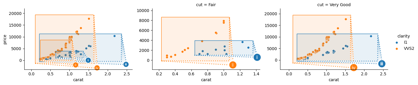
Passing different keys OutsetGrid(col="cut", hue="clarity") will facet on both keys, rendering several hue-mapped marquees per outset frame.
Explicit Zoom Areas
[8]:
# adapted from https://seaborn.pydata.org/examples/wide_data_lineplot.html

# --- Data Preparation ---
# Create a random state and generate a DataFrame with cumulative sum values.
values = np.random.RandomState(365).randn(365, 4).cumsum(axis=0)
dates = np.array(range(365))
data = pd.DataFrame(values, dates, columns=["A", "B", "C", "D"])
data = data.rolling(7).mean()  # Apply a rolling mean with a 7-day window.

# --- Plot Initialization ---
# Initialize an OutsetGrid object with explicit marquee position
outset_grid = otst.OutsetGrid(
    aspect=2,
    data=[(210, 6, 250, 12)],  # Explicit marquee positioning.
    col_wrap=1,  # Ensure vertical layout (two rows)
    x="days",
    y="profit",
)

# --- Broadcast Plotter ---
# Broadcast a line plot over all axes..
outset_grid.broadcast(
    sns.lineplot,
    data=data,
    linewidth=2.5,
    zorder=-1,  # Ensure the line plot is behind other plot elements.
)

# --- Finalization ---
# Draw marquee elements and conclude the script.
outset_grid.marqueeplot()

pass  # sponge up last return value, if any
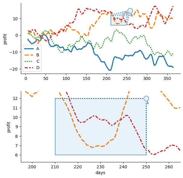
To manually specify zoom frames instead of inferring them from data structure, pass frame coordinates instead of a dataframe when initializing OutsetGrid. In this case, outset.OutsetGrid(data=[(210, 6, 250, 12)]).
Because data is not faceted over plot components, we will need to provide data when rendering plot elements. To manually pass a data kwarg through to the plotting function, use OutsetGrid.broadcast instead of OutsetGrid.map_dataframe. In this case, OutsetGrid.broadcast(sns.lineplot, data=df). The plotter will be called with the same data on each axes, then the subsequent call to marqueeplot will adjust axes data limits to magnify areas specified at OutsetGrid
initialization in outset axes.
[9]:
# adapted from https://seaborn.pydata.org/examples/wide_data_lineplot.html

# --- Data Preparation ---
# Create a random state and generate a DataFrame with cumulative sum values.
values = np.random.RandomState(365).randn(365, 4).cumsum(axis=0)
dates = np.array(range(365))
data = pd.DataFrame(values, dates, columns=["A", "B", "C", "D"])
data = data.rolling(7).mean()  # Apply a rolling mean with a 7-day window.

# --- Plot Initialization ---
# Initialize an OutsetGrid object to create line and scatter plots.
outset_grid = otst.OutsetGrid(
    aspect=2,
    data=[(210, 6, 250, 12)],  # explicit marquee positioning
    col_wrap=1,  # Ensure vertical layout (two rows)
    x="days",
    y="profit",
)

# --- Broadcast Plotter ---
# Broadcast a line plot over all axes .
outset_grid.broadcast(
    sns.lineplot,
    data=data,
    linewidth=otst.util.SplitKwarg(source=2.5, outset=10),  # Line width.
    zorder=-1,  # Ensure the line plot is behind other plot elements.
)

# Broadcast a scatter plot to highlight specific data points.
outset_grid.broadcast_source(
    sns.scatterplot,
    data=data[::20],  # Data points to highlight.
    zorder=-1,  # Ensure the scatter plot is behind other plot elements.
    s=50,  # Marker size.
)

# --- Finalization ---
# Apply additional plot settings and draw marquee elements.
outset_grid.broadcast_outset(lambda: plt.axis("off"))  # Turn off axis.
outset_grid.marqueeplot()  # Draw marquee elements.

pass  # sponge up last return value, if any
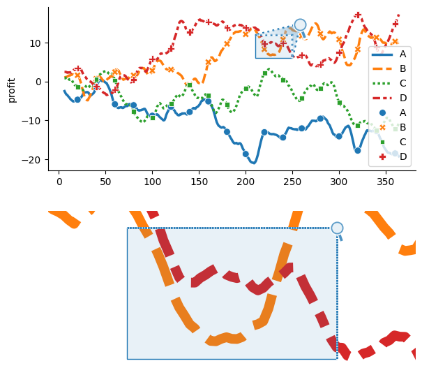
Source axes and outset axes can be targeted in isolation using OutsetGrid.broadcast_source and OutsetGrid.broadcast_outset methods. These work equivalently to OutsetGrid.broadcast, except only dispatch the plotter to the source or outset axes, respectively. For scenarios where an individual kwarg’s value should differ between source and outset axes, OutsetGrid.broadcast may be used in conjuction with the outset.util.SplitKwarg utility. In the example above, for instance,
SplitKwarg is used to differentiate line width between source and outset axes, OutsetGrid.broadcast(sns.lineplot, linewidth=otst.util.SplitKwarg(source=2.5, outset=10)).
(Equivalent OutsetGrid.map_dataframe_source and OutsetGrid.map_dataframe_outset methods are also available for the data-driven OutsetGrid interface, and OutsetGrid.map_dataframe is compatible with SplitKwarg.)
Aspect Ratio
As much fun as we might have with narrow and/or wide Grace Hopper…
[10]:
# --- Data Preparation ---
# Load the sample image of Grace Hopper.
with mpl_cbook.get_sample_data("grace_hopper.jpg") as image_file:
    image = plt.imread(image_file)

# --- Plot Initialization ---
# Initialize a subplot with 1 row and 2 columns.
fig, axs = plt.subplots(1, 2)

# --- Image Display with Bad Aspects ---
# Display the image with an exaggerated aspect ratio.
axs[0].imshow(image, aspect=7, extent=(0, 1, 0, 1), origin="upper", zorder=-1)
axs[0].set_axis_off()  # Remove the axis for a cleaner look.

# Display the image with a compressed aspect ratio.
axs[1].imshow(image, aspect=0.3, extent=(0, 1, 0, 1), origin="upper", zorder=-1)
axs[1].set_axis_off()  # Remove the axis for a cleaner look.

pass  # sponge up last return value, if any
… usually we want to make sure images keep their natural aspect ratio. Luckily, OutsetGrid can take care of that for us.
[11]:
# adapted from https://seaborn.pydata.org/examples/scatter_bubbles.html

# --- Data Preparation ---
# Load the 'mpg' dataset and remove any missing values.
data = sns.load_dataset("mpg").dropna()

# --- Plot Initialization ---
# Initialize an OutsetGrid object to create a scatter plot with bubble sizes.
outset_grid = otst.OutsetGrid(
    data=[(73.5, 23.5, 78.5, 31.5)],  # Explicit marquee positioning.
    color=sns.color_palette()[-1],  # Set color for the marquee.
    marqueeplot_kws={
        "mark_glyph": otst.mark.MarkAlphabeticalBadges(
            start="A",  # Uppercase alphabetical identifiers.
        ),
        "frame_outer_pad": 0.2,
        "frame_outer_pad_unit": "inches",
        "frame_face_kws": {"facecolor": "none"},  # Transparent frame.
    },
)

# --- Broadcast Plotter ---
# Broadcast a scatter plot to visualize 'horsepower' vs 'mpg' with bubble sizes representing 'weight'.
outset_grid.broadcast(
    sns.scatterplot,
    data=data,
    x="horsepower",
    y="mpg",
    hue="origin",  # Color by 'origin'.
    size="weight",  # Size bubbles by 'weight'.
    sizes=(40, 400),  # Range of bubble sizes.
    alpha=0.5,  # Transparency of bubbles.
    palette="muted",  # Color palette.
    zorder=0,  # Z-order for layering.
)

# --- Finalization ---
# Draw marquee elements and set plot titles.
outset_grid.marqueeplot(equalize_aspect=False)
outset_grid.add_legend()
outset_grid.set_titles("")

pass  # sponge up last return value, if any
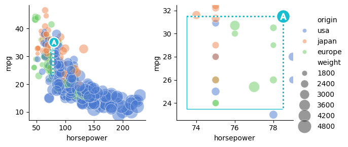
Because synchronized aspect ratios benefit intuitive comparison between outsets and the source plot, under default settings OutsetGrid operations automatically apply corrections to provide equivalent aspect ratios across the source and outset plots. Correction is performed for all plot types, not just images.
The OutsetGrid map dataframe, broadcast, and insetting methods equalize aspect ratio among axes, if necessary, before returning. If you perform other operations that might distort aspect ratios (e.g., adding a legend, stripping axes ticks, etc.) you should call OutsetGrid.equalize_aspect directly at the end of plotting to re-sync aspect ratios
In cases where mismatching aspect ratios are desired — for example, to allow for “better” zoom when aspect is narrow — use the OutsetGrid.marqueeplot(equalize_aspect=False) kwarg.
[12]:
# --- Data Preparation ---
# Load the sample image of Grace Hopper.
with mpl_cbook.get_sample_data("grace_hopper.jpg") as image_file:
    image = plt.imread(image_file)

h, w = image.shape[0], image.shape[1]

# --- Plot Initialization ---
# Initialize an OutsetGrid object for displaying the image with specific marquee frames.
outset_grid = otst.OutsetGrid(
    data=otst.util.NamedFrames(
        {
            # Coordinates for the 'hat' marquee.
            "hat": (0.42 * w, 0.78 * h, 0.62 * w, 0.98 * h),
            # Coordinates for the 'badge' marquee.
            "badge": (0.10 * w, 0.14 * h, 0.40 * w, 0.21 * h),
        }
    ),
    col="swag",  # Name for column mapping (used in titles)
    hue="swag",  # Name for Hue mapping (used in legends)
    aspect=w / h,  # match image aspect
)

# --- Image Display ---
# Turn off the axis and display the image with specified z-order and origin.
outset_grid.broadcast(lambda: plt.axis("off"))
outset_grid.broadcast(
    plt.imshow, image, extent=(0, w, 0, h), origin="upper", zorder=-1
)

# --- Finalization ---
# Draw marquee elements and set the title for the source axes.
outset_grid.source_axes.set_title("The Hopster", loc="left")
outset_grid.marqueeplot(preserve_aspect=True)

pass  # sponge up last return value, if any
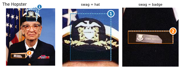
Default aspect ratio synchronization among axes will ensure aspect ratios match, but original aspect ratios may not be preserved under map, broadcast, and insetting methods. To keep a specific aspect ratio, like you might want when working with an image, pass the OutsetGrid(preserve_aspect=True) kwarg.
Layout Control
[13]:
# --- Plot Initialization ---
# Initialize an OutsetGrid object to create KDE plots for the 'iris' dataset.
outset_grid = otst.OutsetGrid(
    data=sns.load_dataset("iris").dropna(),
    x="petal_width",
    y="petal_length",
    col="species",  # Separate plots by species.
    col_wrap=2,  # Display plots in 2 columns, multiple rows
    color=sns.color_palette()[1],  # Set color for the marquee.
    marqueeplot_kws={
        "mark_glyph": otst.mark.MarkAlphabeticalBadges,
    },  # Alphabetical identifiers, lowercase,
    marqueeplot_source_kws={  # Reorient marquee annotations on source axes
        "leader_tweak": otst.tweak.TweakReflect(),
    },
    marqueeplot_outset_kws={  # Reorient marquee annotations on outset axes
        "leader_tweak": otst.tweak.TweakReflect(vertical=True),
    },
)

# --- Map KDE Plot over faceted data ---
# Map KDE plots separately for source and outset data.
outset_grid.map_dataframe_source(
    sns.kdeplot, x="petal_width", y="petal_length", legend=False, zorder=0
)
outset_grid.map_dataframe_outset(
    sns.kdeplot,
    x="petal_width",
    y="petal_length",
    fill=True,
    legend=False,
    zorder=0,
)

# --- Finalization ---
# Draw marquee elements.
outset_grid.marqueeplot()

pass  # sponge up last return value, if any
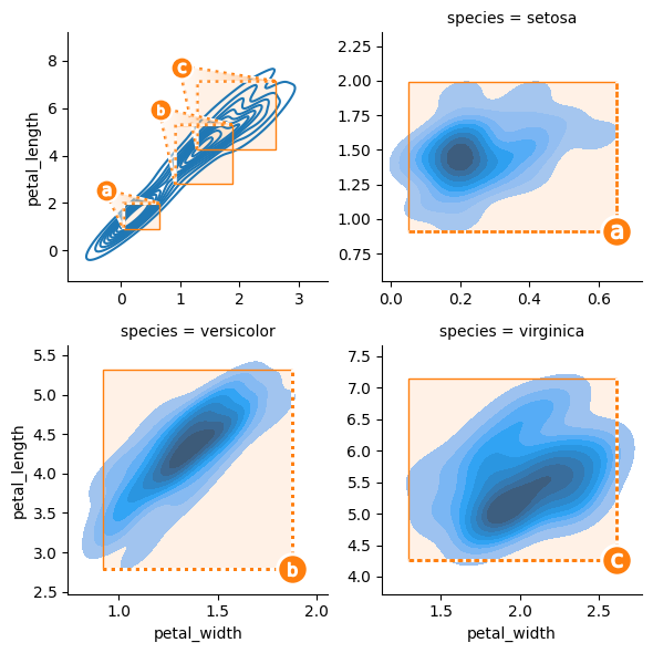
Marquee styling is controlled by passing content via the OutsetGrid.__init__(marqueeplot_kws=dict()) kwarg.
Notable options include marqueeplot_kws=dict(mark_glyph=outset.mark.MarkAlphabeticalBadges) to switch from numerical marquee identifiers to alphabetical identifiers. Use marqueeplot_kws=dict(leader_tweak=outset.tweak.TweakReflect(horizontal=True)) to flip the orientation of marque identifiers. (The TweakReflect functor also accepts a vertical kwarg.)
[14]:
# --- Plot Initialization ---
# Initialize an OutsetGrid object to create scatter plots for the 'penguins' dataset.
outset_grid = otst.OutsetGrid(
    data=sns.load_dataset("penguins").dropna(),
    x="bill_length_mm",
    y="bill_depth_mm",
    col="island",  # Separate plots by island.
    col_order=["Biscoe", "Dream"],  # Order of islands to display.
    hue="species",  # Color by species.
    marqueeplot_kws={
        "mark_glyph": otst.mark.MarkRomanBadges
    },  # Roman numeral identifiers.
    marqueeplot_source_kws={
        "leader_face_kws": {"alpha": 0.2},
        # Push marquee identifiers apart from crowded area
        "leader_tweak": otst.tweak.TweakSpreadArea(
            spread_factor=(2.6, 2.5),
            xlim=(45.5, 52),
            ylim=(21, 24),
        ),
    },
)

# --- Map Scatter Plot over faceted data ---
# Map scatter plots for 'bill_length_mm' vs 'bill_depth_mm'.
outset_grid.map_dataframe(
    sns.scatterplot, x="bill_length_mm", y="bill_depth_mm", legend=False
)

# --- Finalization ---
# Draw marquee elements, set axis labels, and add a legend.
outset_grid.marqueeplot()
outset_grid.set_axis_labels("bill length (mm)", "bill depth (mm)")
outset_grid.add_legend()

pass  # sponge up last return value, if any
No artists with labels found to put in legend. Note that artists whose label start with an underscore are ignored when legend() is called with no argument.
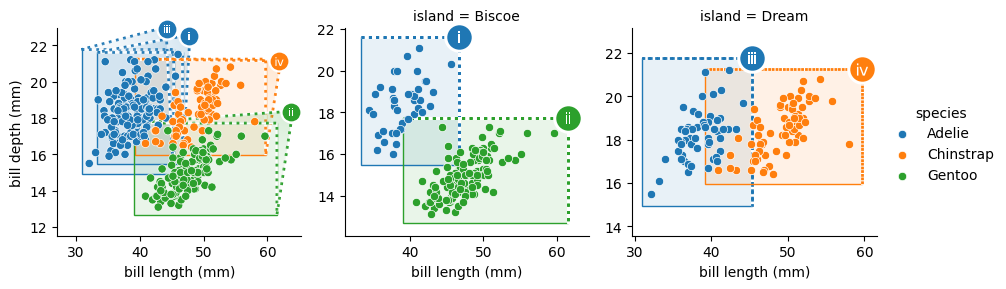
The TweakSpreadArea functor is available to resolve collisions between marquee identifying marks by spreading marks within a designated area apart. In this case,
OutsetGrid(
    marqueeplot_source_kws={
        "leader_tweak": otst.tweak.TweakSpreadArea(
            spread_factor=(2.6, 2.5),
            xlim=(45.5, 52),
            ylim=(21, 24),
        ),
    },
)
pushes the i and iii markers apart.
See documentation for outset.marqueeplot, outset.draw_marquee, or the gallery page to see additional available styling and layout options.
[15]:
# --- Plot Initialization ---
# Initialize an OutsetGrid object to create KDE plots for the 'iris' dataset.
outset_grid = otst.OutsetGrid(
    data=sns.load_dataset("iris").dropna(),
    x="petal_width",
    y="petal_length",
    col="species",  # Separate plots by species.
    color=sns.color_palette()[1],  # Set color for the marquee.
    marqueeplot_kws={
        "mark_glyph": otst.mark.MarkAlphabeticalBadges,
    },  # Alphabetical identifiers, lowercase,
    marqueeplot_source_kws={  # Reorient marquee annotations on source axes
        "leader_tweak": otst.tweak.TweakReflect(),
    },
    marqueeplot_outset_kws={  # Reorient marquee annotations on outset axes
        "leader_tweak": otst.tweak.TweakReflect(vertical=True),
    },
)

# --- Map KDE Plot over faceted data ---
# Map KDE plots separately for source and outset data.
outset_grid.map_dataframe_source(
    sns.kdeplot, x="petal_width", y="petal_length", legend=False, zorder=0
)
outset_grid.map_dataframe_outset(
    sns.kdeplot,
    x="petal_width",
    y="petal_length",
    fill=True,
    legend=False,
    zorder=0,
)

# --- Finalization ---
otst.inset_outsets(outset_grid, "SE")  # move outsets into lower right of source
outset_grid.marqueeplot()  # Draw marquee elements.

pass  # sponge up last return value, if any
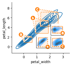
Any OutsetGrid can be transformed into an inset plot through outset.inset_outsets. This function takes an OutsetGrid as an argument, and rearranges it to reposition outset axes directly over the source plot axes. The corner to place outset axes in can be designated as NE (upper right), SE (lower right), etc., like outset.inset_outsets(outset_grid, "SE").
Several levels of abstraction are available to decide inset geometry — a call to outset.util.layout_corner_insets or even hard axes-relative coordinates can be provided in place of a cardinal corner designation. See the gallery for examples.
Axes-level Interfaces
Most use cases should only need OutsetGrid, but outset does make more granular control available through lower-level APIs.
[16]:
# --- Plot Initialization ---
# Initialize a subplot.
fig, ax = plt.subplots(1)

# --- Marquee Plotting ---
# Create a marquee plot with the 'iris' dataset.
otst.marqueeplot(
    data=sns.load_dataset("iris"),
    x="petal_length",
    y="petal_width",
    hue="species",  # Color by species.
    ax=ax,  # Specify the axis for plotting.
    leader_stretch=0.4,  # Stretch factor for leaders.
    leader_tweak=otst.tweak.TweakReflect(
        vertical=True
    ),  # Tweak leaders for better visibility.
)

# --- Scatter Plot ---
# Overlay a scatter plot on the same axes.
sns.scatterplot(
    data=sns.load_dataset("iris"),
    x="petal_length",
    y="petal_width",
    hue="species",  # Color by species.
    ax=ax,  # Specify the axis for plotting.
)

pass  # sponge up last return value, if any
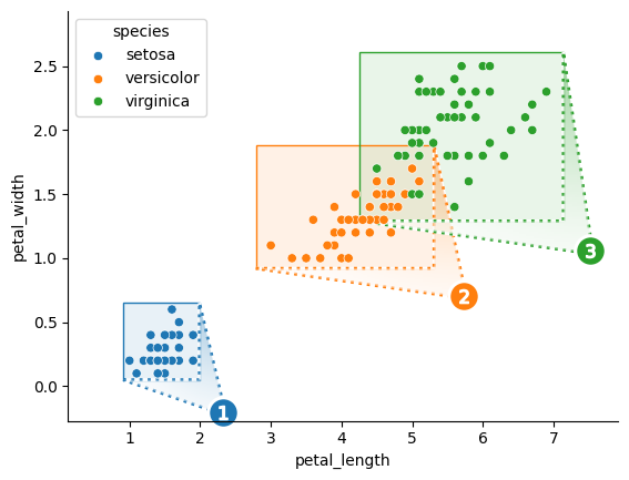
Use marqueeplot for seaborn-like, data-oriented application of marquee annotations to a single Axes. (This function determines frame positions according to the x/y extents of data subsets.)
[17]:
# adapted from https://seaborn.pydata.org/examples/smooth_bivariate_kde.html

# --- Plot Initialization ---
# Initialize a subplot.
fig, ax = plt.subplots(1)

# --- KDE Plotting ---
# Create a KDE plot of body mass vs. bill depth for the penguins dataset.
sns.kdeplot(
    data=sns.load_dataset("penguins"),
    x="body_mass_g",
    y="bill_depth_mm",
    ax=ax,
    fill=True,
    clip=((2200, 6800), (10, 25)),  # Limit the data to a specific range.
    thresh=0,
    levels=100,  # Set the number of contour levels.
    cmap="rocket",  # Color map.
)

# --- Marquee Annotation ---
# Draw a  single marquee around a specific region of interest.
otst.draw_marquee(
    (5200, 6000),  # X range for the marquee.
    (14, 16),  # Y range for the marquee.
    ax,
    color="teal",  # Color of the marquee.
    mark_glyph=otst.mark.MarkArrow(rotate_angle=-45),  # Marquee identifier
    leader_stretch_unit="inches",
    leader_stretch=0.2,  # Stretch factor for leaders.
    zorder=10,
)

# --- Annotation ---
# Add a fun text annotation.
ax.annotate("zoink?", (6300, 17), color="teal", zorder=5)

pass  # sponge up last return value, if any
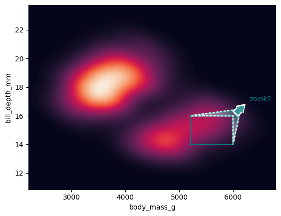
Use draw_marquee to manually add individual annotations.
Further Subjects
The class OutsetGrid inherits from seaborn.FacetGrid, which provides a rich set of initializer kwargs and member properties/functions available to the end user. See the README and examples in the gallery for examples demonstrating these customization capabilities, as well as the full range of styling customization capabilities available.
Some caveats and known limitations should be noted.
Try to call
OutsetGrid.marqueeplotlater rather than earlier — the layout algorithms make use of information about current axes state to determine positioning and sizing of annotation elements.OutsetGridconstruction can sometimes be sensitive to operation order, especially when generating colorbars and legends. Again, refer to gallery for examples with working operation orders.Inverted axes are currently not supported.
See here for an example involving log-scale axes.
Finally, if this code is useful to you, please consider leaving a ⭐ on GitHub. Thanks!