Profiling Foundations for Scalable Digital Evolution Methods
contents
Digital evolution techniques complement traditional wet-lab evolution experiments by enabling researchers to address questions that would be otherwise limited by:
- reproduction rate (which determines the number of generations that can be observed in a set amount of time),
- incomplete observations (every event in a digital system can be tracked),
- physically-impossible experimental manipulations (every event in a digital system can be arbitrarily altered), or
- resource- and labor-intensity (digital experiments and assays can be easily automated).
The versatility and rapid generational turnover of digital systems can easily engender a notion that such systems can already operate at scales greatly exceeding biological evolution experiments. Although digital evolution techniques can feasibly simulate populations numbering in the millions or billions, doing so requires very simple agents and/or very limited agent-agent interaction. With more complex agents controlled by genetic programs, neural networks, or the like, feasible population sizes dwindle down to thousands or hundreds of agents.
🔗 Putting Scale in Perspective
Take Avida as an example. This is a popular software system that enables experiments with evolving self-replicating computer programs. In this system, a population of ten thousand can undergo about twenty thousand generations per day. This means that about two hundred million replication cycles are performed in a day [Ofria et al., 2009].
Each flask in the Lenski Long-Term Evolution Experiment hosts a similar number of replication cycles. In their system, E. coli undergo about six doublings per day. Effective population size is reported as 30 million [Good et al., 2017]. Hence, about 180 million replication cycles elapse per day.
Likewise, in Ratcliff’s work studying the evolution of multicellularity in S. cerevisiae, about six doublings per day occur among a population numbering on the order of a billion cells [Ratcliff, 2012]. So, around six billion cellular replication cycles elapse per day in this system.
Although artificial life practitioners traditionally describe instances of their simulations as “worlds,” with serial processing power their scale aligns (in naive terms) more along the lines of a single flask. Of course, such a comparison neglects the disparity between Avidians and bacteria or yeast in terms of genome information content, information content of cellular state, and both quantity and diversity of interactions with the environment and with other cells.
Recent work with SignalGP has sought to address some of these shortcomings by developing digital evolution substrates suited to more dynamic environmental and agent-agent interactions [Lalejini and Ofria, 2018] that more effectively incorporate state information [Lalejini et al., 2020; Moreno, 2020]. However, to some degree, more sophisticated and interactive evolving agents will necessarily consume more CPU time on a per-replication-cycle basis — further shrinking the magnitude of experiments tractable with serial processing.
🔗 The Future is Plastics Parallel
Throughout the 20th century, serial processing enjoyed regular advances in computational capacity due to quickening clock cycles, burgeoning RAM caches, and increasingly clever packing together of instructions during execution. Since, however, performance of serial processing has bumped up against apparent fundamental limits to computing’s current technological incarnation [Sutter, 2005]. Instead, advances in 21st century computing power have arrived via multiprocessing [Hennessy and Patterson, 2011, p.55] and hardware acceleration (e.g., GPU, FPGA, etc.) [Che et al., 2008].
Contemporary high-performance computing clusters link multiprocessors and accelerators with fast interconnects to enable coordinated work on a single problem [Hennessy and Patterson, 2011, p.436]. High-end clusters already make hundreds of thousands or millions of cores available. More loosely-affiliated banks of servers can also muster significant computational power. For example, Sentient Technologies notably employed a distributed network of over a million CPUs to run evolutionary algorithms [Miikkulainen et al., 2019].
The availability of orders of magnitude greater parallel computing resources in ten and twenty years’ time seems probable, whether through incremental advances with traditional silicon-based technology or via emerging, unconventional technologies such as bio-computing [Benenson, 2009] and molecular electronics [Xiang et al., 2016]. Such emerging technologies could make greatly vaster collections of computing devices feasible, albeit at the potential cost of component-wise speed [Bonnet et al., 2013; Ellenbogen and Love, 2000] and perhaps also component-wise reliability.
🔗 What of Scale?
Parallel and distributed computing has long been intertwined with digital evolution [Moreno and Ofria, 2020]. Practitioners typically proceed along the lines of the island model, where subpopulations evolve in parallel with intermittent exchange of individuals [Bennett III et al., 1999]. Similarly, in scientific contexts, absolute segregation is often enforced between parallel subpopulations to yield independent replicate datasets [Dolson and Ofria, 2017].
These techniques can enable observation of rare events and provide statistical power to answer research questions. However, evolving subpopulations in parallel does not lend itself to large-scale study of interaction-driven phenomena such as
- multicellularity,
- sociality, and
- ecologies.
These topics are of interest in digital evolution and artificial life, particularly with respect to the issue of open-ended evolution. While by no means certain, it seems plausible that orders-of-magnitude increases in system scale will enable qualitatively different experimental possibilities [Moreno and Ofria, 2020].
So, how can we exploit parallel computing power in digital evolution systems revolving around such interaction-driven phenomena? Addressing this question will be key both to enabling digital evolution to take full advantage of already-available contemporary computational resources and to positioning digital evolution to exploit vast computational resources that will likely become available in the not-too-distant future.
🔗 Model Choice
In this blog series, we will investigate the scaling properties of a std::thread/MPI-based implementation of an asynchronous cellular automata model.
Our immediate goal is to establish a foundation for continuing work [Moreno, 2020] building a scalable implementation of the DISHTINY framework for studying digital multicellularity [Moreno and Ofria, 2020; Moreno and Ofria, in prep.; Moreno and Ofria, 2019]. Although the exact formulation is unimportant for the purposes of these writeups, the system might be loosely described along the lines of a grid-based cellular automata where the rule set itself is transmissible (i.e., a genetic program).
The underlying design of DISHTINY and choice of the model system profiled here is motivated by David Ackley’s notion of indefinite scalability [Ackley, 2011]. In order to meaningfully function with arbitrarily large numbers of computational nodes, he argues, a system must respect:
- asynchrony,
- fault-tolerance, and
- spatial locality.
Any system operating within Ackley’s framework for indefinite scalability must at least bear a passing resemblance to an asynchronous cellular automata. So, hopefully, software tools developed and profiling results reported here might be of broader interest to researchers developing scalable artificial chemistry and artificial life simulations.
🔗 Software Abstraction
The backbone of the prototype implementation is a “Pipe” model consisting of an Inlet, a Duct, and an Outlet.
Data is deposited via the Inlet, transmitted via the Duct, and received via the Outlet.
Figure SOOPC outlines how these components relate.
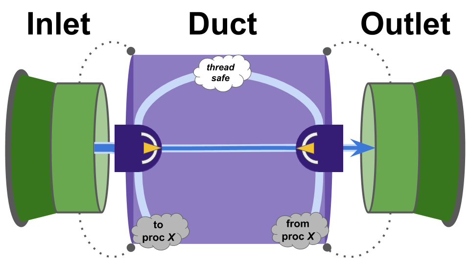 Figure SOOPC:
Schematic overview of pipe components.
Figure SOOPC:
Schematic overview of pipe components.
API interaction occurs exclusively via the Inlet and the Outlet — not directly with the Duct.
The Duct’s underlying transmission mechanism can be changed from intra-thread transmission to inter-thread or inter-process transmission through either the Inlet or the Outlet.
Under the hood, an Inlet and Outlet hold a std::shared_ptr to a Duct.
So, either the Inlet or the Outlet can be deleted while the Duct remains (as might be useful in the case of an inter-process duct).
The Duct contains a std:variant of the underlying transmission mechanisms.
This way, the underlying transmission mechanism can be changed out in-place.
Send operations into the Inlet are non-blocking.
However, as shown in Figure SOOIF, in the current implementation if the Inlet’s buffer capacity has been reached, the send operation may drop.
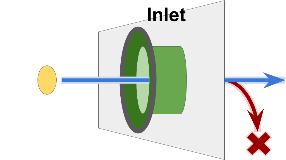 Figure SOOIF:
Schematic overview of
Figure SOOIF:
Schematic overview of Inlet function.
Likewise, receive operations from the Outlet are non-blocking.
A receive operation returns the most recently received value via the Duct.
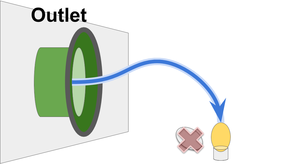 Figure SOOOF:
Schematic overview of
Figure SOOOF:
Schematic overview of Outlet function.
This software design aims to hide the complexity of wiring data between heterogeneous computational elements.
As shown in Figure AUIFC, the exact same interface — Inlets and Outlets — performs communication within threads, between threads, or between processes.
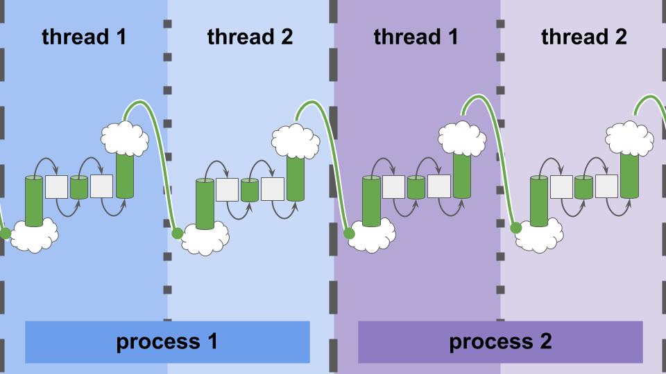 Figure AUIFC:
A uniform interface for communication within-thread, between-threads, and between-processes.
Figure AUIFC:
A uniform interface for communication within-thread, between-threads, and between-processes.
Intra-process message passing (accomplished via MPI [Clarke et al., 1994]) allows systems built with this infrastructure to span across compute nodes.
🔗 Model System
Using this “Pipe” API, we construct a simple one-dimensional cellular automata for use in profiling experiments.
Two states are possible.
At each update, cells adopt the state of their left neighbor — read through an Outlet.
States are initialized randomly.
Figure ASODC summarizes.
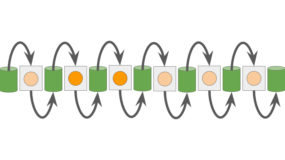 Figure ASODC:
A simple one-dimensional cellular automata.
Figure ASODC:
A simple one-dimensional cellular automata.
🔗 Scaling Memory & Compute
The amount of memory used per unit of computational work is crucial to the performance characteristics of software — and varies widely between applications. Because our goal is to characterize the general scaling properties of our asynchronous communication implementation, we need to test broadly across memory-to-compute ratios.
As shown in Figure MPVCO, there are two levers we can pull to increase the amount of computational work in our model system.
- We can increase the number of tiles in our one-dimensional grid. This increases memory use in proportion with compute.
- We can increase the amount of computational work performed per tile update.
This increases compute load without affecting memory use.
(Under the hood this computational work is just increasing numbers of calls to a
thread_localpseudorandom number generator.)
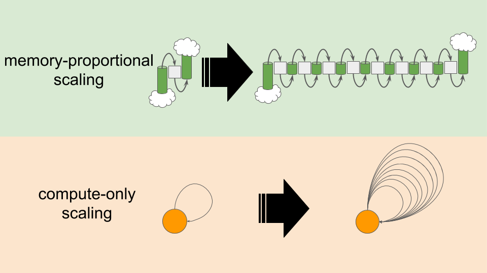 Figure MPVCO:
Memory-proportional versus compute-only scaling.
Figure MPVCO:
Memory-proportional versus compute-only scaling.
We use these two levers to perform scaling experiments along six trajectories:
- compute-lean,
- memory-proportional scaling with minimal computational cost per tile update
- increasing grid size with 1 RNG call per tile update
- compute-moderate,
- memory-proportional scaling with moderate computational cost per tile update
- increasing grid size with 64 RNG calls per tile update
- compute-intensive,
- memory-proportional scaling with intensive computational cost per tile update
- increasing grid size with 4096 RNG calls per tile update
- memory-lean,
- compute-only scaling with low memory use
- increasing RNG calls per tile update with 1 grid tile
- memory-moderate, and
- compute-only scaling with moderate memory use
- increasing RNG calls per tile update with 64 grid tiles
- memory-intensive.
- compute-only scaling with intensive memory use
- increasing RNG calls per tile update with 4096 grid tiles
Figure SSTIC summarizes the relationship of these scaling trajectories in memory-compute space.
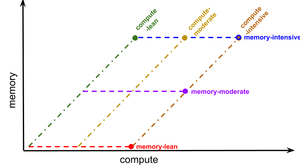 Figure SSTIC:
Six scaling trajectories in compute-memory space.
Each trajectory is represented as a uniquely-colored line.
The bulb end indicates the end of the trajectory.
Figure SSTIC:
Six scaling trajectories in compute-memory space.
Each trajectory is represented as a uniquely-colored line.
The bulb end indicates the end of the trajectory.
🔗 Single-Core Scaling
In order to provide a baseline characterization of our model system and our experimental scaling methods, we start by evaluating serial performance along each of our scaling trajectories. We measure the amount of work performed in terms of the number of RNG calls dispatched.
Figure CWRAT shows work rate along each scaling trajectory.
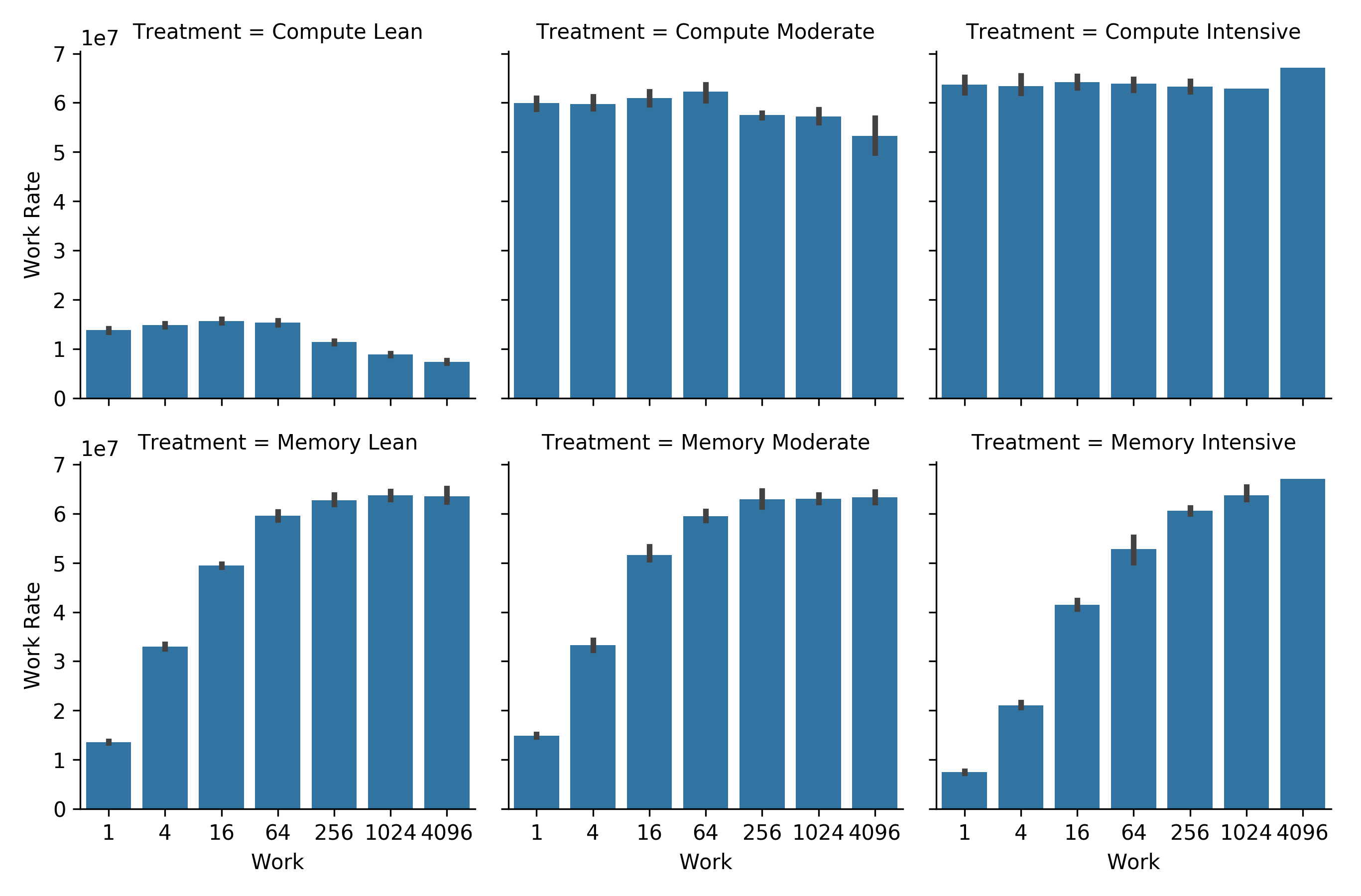 Figure CWRAT:
Computational work rate along the scaling trajectories described in Figure SSTIC.
Sequential bars represent increasing total work.
Along the top row, computational work and memory usage increase proportionally.
Along the bottom row, computational work increases but memory usage does not.
Error bars represent bootstrapped 95% confidence intervals.
Figure CWRAT:
Computational work rate along the scaling trajectories described in Figure SSTIC.
Sequential bars represent increasing total work.
Along the top row, computational work and memory usage increase proportionally.
Along the bottom row, computational work increases but memory usage does not.
Error bars represent bootstrapped 95% confidence intervals.
On the bottom row, the work rate increases as more computational work is performed per tile update. Exactly as expected — with more work per update a smaller and smaller fraction of time is spent communicating between grid cells and refreshing cell state.
On the top row, at low computational load (computational lean and moderate), increasing grid size decreases performance. This could be due to memory locality worsening under a larger memory footprint — when more memory sites are touched, cache is not as effective.
🔗 Memory Locality
In order to further investigate the hypothesis of worsening memory locality as grid size increases at low computational load, we tried distributing work between threads on our single-core allocation. Figure STEOA shows grid size before multithreading and Figure MTEOA shows grid size after multithreading.
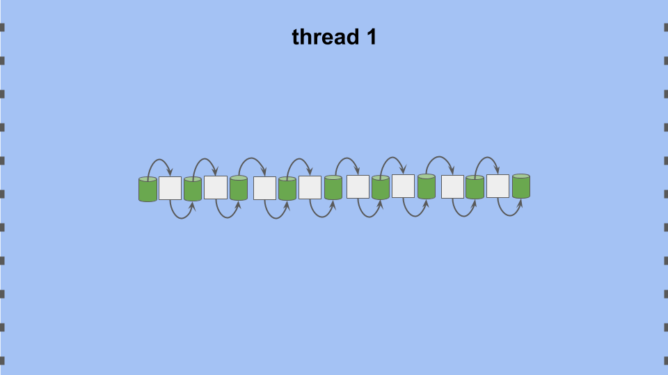 Figure STEOA:
Single-threaded evaluation of an eight-tile cellular automata.
Figure STEOA:
Single-threaded evaluation of an eight-tile cellular automata.
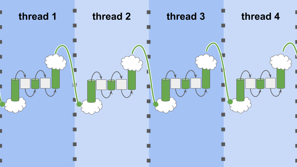 Figure MTEOA:
Multi-threaded evaluation of an eight-tile cellular automata.
Each thread only evaluates two tiles.
Figure MTEOA:
Multi-threaded evaluation of an eight-tile cellular automata.
Each thread only evaluates two tiles.
If memory locality was harming performance, we would expect the work rate to improve under multithreading because each thread has a smaller memory footprint. (Although overhead of thread creation and thread switching might potentially counteract this effect.)
Here, we consider the most memory-intense scaling trajectories from Figure SSTIC — where we would be most likely to observe a memory locality effect. In Figure NWRCL, work rate increases with thread count at the end of the compute-lean scaling trajectory, where memory intensity is greatest. Likewise, in Figure NWRMI, work rate increases with thread count at the beginning of the memory-intensive scaling trajectory, where memory intensity is also greatest.
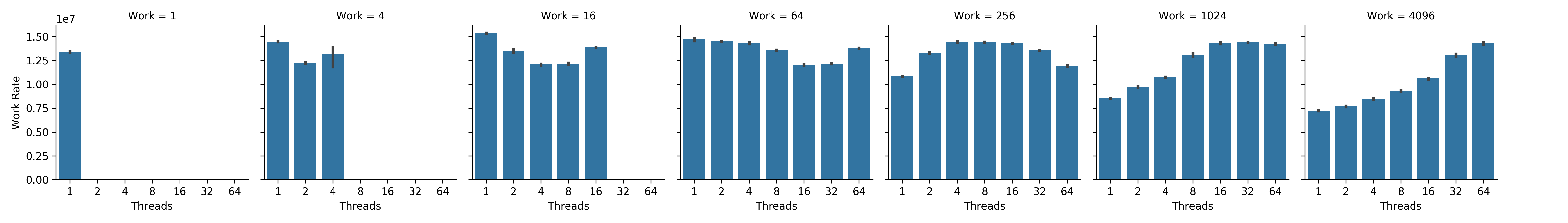 Figure NWRCL:
Net work rate by thread count at different total work loads along the compute-lean scaling trajectory.
Subplots correspond left to right to increasing total work load.
Bars within subplots correspond left to right to increasing thread count.
Error bars represent bootstrapped 95% confidence intervals.
Figure NWRCL:
Net work rate by thread count at different total work loads along the compute-lean scaling trajectory.
Subplots correspond left to right to increasing total work load.
Bars within subplots correspond left to right to increasing thread count.
Error bars represent bootstrapped 95% confidence intervals.
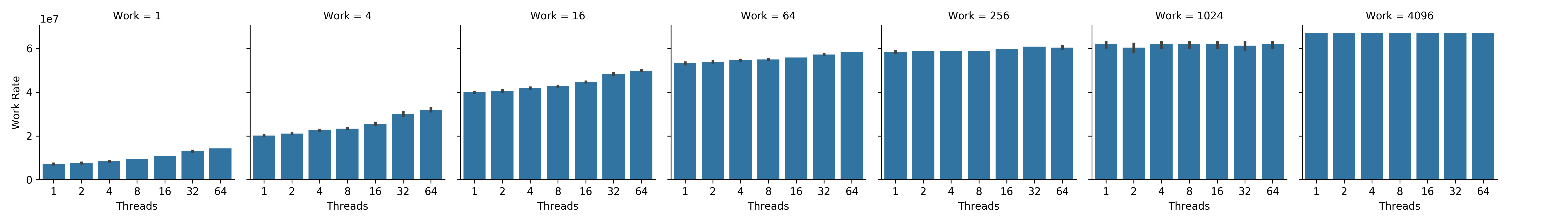 Figure NWRMI:
Net work rate by thread count at different total work loads along the memory-intensive scaling trajectory.
Subplots correspond left to right to increasing total work load.
Bars within subplots correspond left to right to increasing thread count.
Error bars represent bootstrapped 95% confidence intervals.
Figure NWRMI:
Net work rate by thread count at different total work loads along the memory-intensive scaling trajectory.
Subplots correspond left to right to increasing total work load.
Bars within subplots correspond left to right to increasing thread count.
Error bars represent bootstrapped 95% confidence intervals.
These results align with the hypothesis that memory locality effects are at play. So, we have evidence that the range of memory intensities laid out for our scaling experiments is adequately broad to be representative of more memory-bound applications. In addition, it suggests the possibility that with an asynchronous approach we ultimately may be able to achieve a speedup by creating more threads than available cores to reduce per-thread work load and improve memory locality.
🔗 Don’t Touch That Dial!
We’ve reached the end of this blog post. We’ve motivated and introduced the software design and evaluation methodology used, but there’s still much to cover!
Upcoming material will describe,
- measuring efficiency of multithreaded and multiprocess scaling,
- measuring the distribution of message latency across threads and processes, and
- considering the effects of message size and volume.
Stay tuned!
🔗 Cite This Post
APA
Moreno, M. A. (2020, July 7). Profiling Foundations for Scalable Digital Evolution Methods. Retrieved from osf.io/tcjfy
MLA
Moreno, Matthew A. “Profiling Foundations for Scalable Digital Evolution Methods.” OSF, 7 July 2020. Web.
Chicago
Moreno, Matthew A. 2020. “Profiling Foundations for Scalable Digital Evolution Methods.” OSF. July 7. doi:10.17605/OSF.IO/TCJFY.
BibTeX
  @misc{Moreno-2020,
  title={Profiling Foundations for Scalable Digital Evolution Methods},
  url={osf.io/tcjfy},
  DOI={10.17605/OSF.IO/TCJFY},
  publisher={OSF},
  author={Moreno, Matthew A},
  year={2020},
  month={Jul}
}
🔗 Let’s Chat!
Questions? Comments?
I started a twitter thread (right below) so we can chat ![]()
![]()
![]()
nothing to see here, just a placeholder tweet 🐦
— Matthew A Moreno (@MorenoMatthewA) October 21, 2018
Pop on there and drop me a line ![]() or make a comment
or make a comment ![]()
🔗 Code & Data
We ran experiments on single-core interactive allocations on MSU ICER’s css nodes.
Profiling results took about four hours to collect.
Data and figures are available via the Open Science Framework at https://osf.io/je7ad/ [Foster and Deardorff, 2017].
Software used for these experiments is available here. We relied on software components from the Empirical C++ Library for Scientific Software [Ofria et al., 2019], MPI [Clarke et al., 1994], and Matplotlib [Hunter, 2007].
🔗 References
Ackley, D. H. and Cannon, D. C. (2011). Pursue robust indefinite scalability. In HotOS.
Moreno, M. A. (2020, May 1). Evaluating Function Dispatch Methods in SignalGP.
Moreno, M. A. (2020, July 8). Estimating DISHTINY Multithread Scaling Properties.
🔗 Acknowledgements
This research was supported in part by NSF grants DEB-1655715 and DBI-0939454, and by Michigan State University through the computational resources provided by the Institute for Cyber-Enabled Research. This material is based upon work supported by the National Science Foundation Graduate Research Fellowship under Grant No. DGE-1424871. Any opinions, findings, and conclusions or recommendations expressed in this material are those of the author(s) and do not necessarily reflect the views of the National Science Foundation.