Estimating DISHTINY Multithread Scaling Properties
contents
This post develops a statistical model of multithread performance to estimate the following scaling properties:
- parallelizable work fraction,
- and threading efficiency.
Then, we analyze DISHTINY profiling data to identify next steps to enhance parallel performance.
🔗 Data Collection
I collected timing data with 1, 2, 4, 8, and 16 threads enabled on a 16 cpu allocation on MSU ICER’s lac-385 node.
Timing data was collected at five “load” (work per thread) levels: 1, 2, 4, 8, and 16.
(Intuition: a one-thread run with load level 16 conducts the same amount of total work as a sixteen-thread run with load level 1.)
Six replicate measurements of each timing were recorded.
I profiled version 53vgh of the DISHTINY software [Moreno and Ofria, 2020], compiled with data collection disabled. This software is built using the Empirical C++ Library [Ofria et al., 2019]. Data was collected using Script OEFFA.
🔗 Statistical Model
🔗 Modeling Execution Time
In a completely ideal scenario, execution \(\mathrm{time}\) of a parallel application would approximate
Assuming only \(\mathrm{fraction␣parallel}\) of \(\mathrm{work}\), execution \(\mathrm{time}\) would follow
Throwing in a fixed \(\mathrm{overhead}\) to execution and considering that threads might only be used at a \(\mathrm{threading␣efficiency}\) fraction of ideal efficacy,
Unit analysis reveals a missing conversion constant,
Adding the necessary conversion constant,
Rearranging, we can write
🔗 Considering Latency
Define \(\operatorname{latency}\) as a function of \(\mathrm{threads}\),
In this sense, \(\operatorname{latency}\) (time per work) is the inverse of productivity (work per time).
Rewriting Equation \(\ref{eqn:complete}\) in terms of \(\operatorname{latency}(\mathrm{threads})\),
🔗 Estimating Latency
If we fix \(\mathrm{threads}\), we can use a General Linear Model (a.k.a., a fancy-talk linear regression) to estimate specific values of \(\mathrm{latency}\) as a coefficient of \(\mathrm{work}\),
🔗 Modeling Latency
With estimates of \(\mathrm{latency}\) in hand for particular values of \(\mathrm{threads}\), we can use another General Linear Model to estimate the relationship between \(\operatorname{latency}\) and inverse \(\operatorname{threads}\),
🔗 Deducing Scaling Properties
How to get from the estimated \(\mathrm{intercept}\) and \(\mathrm{coefficient}\) from Equation \(\ref{eqn:latencyglm}\) to our real underlying properties of interest: \(\mathrm{fraction␣parallel}\), \(\mathrm{fraction␣serial}\), and \(\mathrm{threading␣efficiency}\)?
From Equation \(\ref{eqn:latency}\), we know that
and that
So far we have four unknowns, but only two equations — not yet enough to deduce our properties of interest. We need two more constraints.
Because \(\mathrm{fraction␣serial}\) and \(\mathrm{fraction␣parallel}\) are complementary by definition, we must have
Finally, when running single-threaded we should have
It follows from Equation \ref{eqn:singlethread} and \ref{eqn:complete} that
Combining constraint Equations \ref{eqn:constraint1}, \ref{eqn:constraint2}, \ref{eqn:constraint3}, and \ref{eqn:constraint4}, we can show that
Expressions for \(\mathrm{fraction␣serial}\), \(\mathrm{fraction␣parallel}\), and \(\mathrm{threading␣efficiency}\) in terms of \(\mathrm{intercept}\) and \(\mathrm{coefficient}\) follow readily.
🔗 Algorithm for Estimating Scaling Properties
Script DUMFD uses the following procedure to estimate key scaling properties from execution timing data.
- Independently across replicates, use linear regression between \(\mathrm{time}\) and \(\mathrm{work}\) to estimate \(\mathrm{latency}\) at each thread count.
formula='Time ~ Work'- \(\mathrm{latency}\) is estimated as coefficient of
Work
- Perform linear regression between per-replicate estimated \(\mathrm{latency}\) and \(\frac{1}{\mathrm{threads}}\).
formula='Q("Estimated Latency") ~ Q("Inverse Threads")'- yields an estimated \(\mathrm{coefficient}\) and \(\mathrm{intercept}\)
- Use estimates of \(\mathrm{coefficient}\) and \(\mathrm{intercept}\) to deduce estimates for:
- \(\mathrm{execution␣seconds␣per␣unit␣work}\),
- \(\mathrm{fraction␣serial}\),
- \(\mathrm{fraction␣parallel}\), and
- \(\mathrm{threading␣efficiency}\).
- Evaluate minima and maxima over all four combinations of 95% confidence bound values of \(\mathrm{coefficient}\) and \(\mathrm{intercept}\) to deduce confidence bounds on estimates for:
- \(\mathrm{execution␣seconds␣per␣unit␣work}\),
- \(\mathrm{fraction␣serial}\),
- \(\mathrm{fraction␣parallel}\), and
- \(\mathrm{threading␣efficiency}\).
🔗 Results
🔗 Raw Timings
Figures SSATW and WSALW arrange raw timings to examine strong and weak scaling properties, respectively, of the DISHTINY implementation.
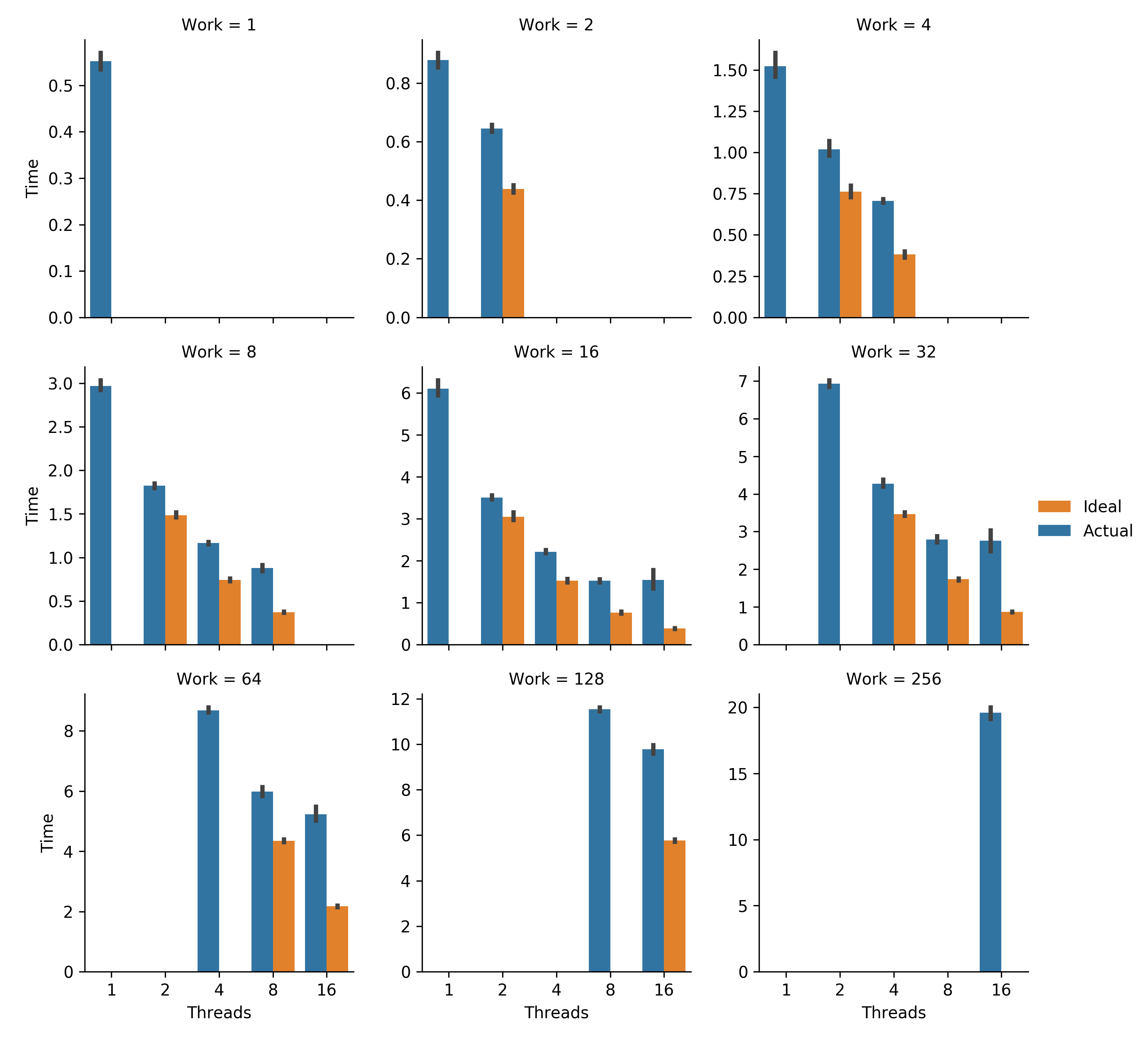 Figure SSATW.
Strong scaling analysis.
Total work remains constant as additional threads are added.
Error bars represent bootstrapped 95% confidence intervals.
Ideal for each work level was calculated as a thread-fraction of the timings of the lowest-threaded trial performed.
Generated via Script AMEAW.
Figure SSATW.
Strong scaling analysis.
Total work remains constant as additional threads are added.
Error bars represent bootstrapped 95% confidence intervals.
Ideal for each work level was calculated as a thread-fraction of the timings of the lowest-threaded trial performed.
Generated via Script AMEAW.
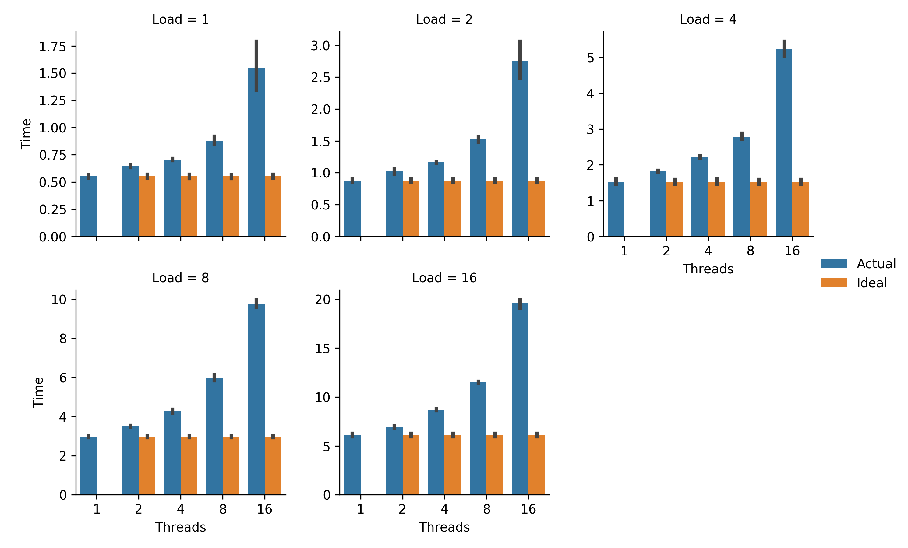 Figure WSALW.
Weak scaling analysis.
Load (work per thread) remains constant as additional threads are used to solve a larger total problem.
Error bars represent bootstrapped 95% confidence intervals.
Ideal for each load level is single-threaded timing.
Generated via Script AMEAL.
Figure WSALW.
Weak scaling analysis.
Load (work per thread) remains constant as additional threads are used to solve a larger total problem.
Error bars represent bootstrapped 95% confidence intervals.
Ideal for each load level is single-threaded timing.
Generated via Script AMEAL.
🔗 Estimated Scaling Properties
Table EOKSP summarizes estimates of key scaling properties of the DISHTINY implementation. Around 85% of work is parallelized. A threading efficiency of around 45% was achieved.
| Parameter | Estimate | Lower Bound | Upper Bound |
|---|---|---|---|
| Parallel Fraction | 0.858 | 0.845 | 0.870 |
| Serial Fraction | 0.142 | 0.130 | 0.155 |
| Threading Efficiency | 0.448 | 0.398 | 0.502 |
Table EOKSP. Estimates of key scaling properties. Upper and lower bounds indicate \(\geq95\%\) confidence. A complete listing of estimated parameters appears in Table EPUAL. Generated via Script DUMFD.
🔗 Discussion
Improving threading efficiency appears the most fruitful approach to improve parallel performance. Only about half threading efficiency appears to currently be achieved. This might be accomplished by reducing synchronization overhead or improving thread memory locality.
Interestingly, threading efficiency appears significantly greater at smaller per-thread loads. This may be due to effects of load size on caching or memory layout. More concretely understanding the cause of this phenomenon may help identify problematic aspects of the existing implementation with respect to multi-threaded performance.
Although the majority of work has been parallelized, remaining serial proportions are statistically detectable. In order to achieve \(>10\times\) speedup, more serial work will have to be parallelized. In particular, this will likely require disabling or reimplementing global systematics tracking.
🔗 Conclusion
By providing estimates for key scaling properties of the DISHTINY system, the statistical model informs our next steps enhancing its parallel performance.
The statistical model developed to estimate scaling properties of interest will provide a framework to quantitatively demonstrate the impact of work to enhance the software’s parallel performance.
Going forward, we should consider constructing a null model to generate simulated timing data. Running this simulated data through our procedure for estimating scaling properties will allow us to confirm the validity of our estimation procedure.
🔗 Cite This Post
APA
Moreno, M. A. (2020, July 6). Estimating DISHTINY Multithread Scaling Properties. https://doi.org/10.17605/OSF.IO/W56BM
MLA
Moreno, Matthew A. “Estimating DISHTINY Multithread Scaling Properties.” OSF, 6 July 2020. Web.
Chicago
Moreno, Matthew A. 2020. “Estimating DISHTINY Multithread Scaling Properties.” OSF. July 6. doi:10.17605/OSF.IO/W56BM.
BibTeX
@misc{Moreno-2020,
  title={Estimating DISHTINY Multithread Scaling Properties},
  url={osf.io/w56bm},
  DOI={10.17605/OSF.IO/W56BM},
  publisher={OSF},
  author={Moreno, Matthew A},
  year={2020},
  month={Jul}
}
🔗 Let’s Chat!
Questions? Comments?
I started a twitter thread (right below) so we can chat ![]()
![]()
![]()
nothing to see here, just a placeholder tweet 🐦
— Matthew A Moreno (@MorenoMatthewA) October 21, 2018
Pop on there and drop me a line ![]() or make a comment
or make a comment ![]()
🔗 References
🔗 Acknowledgements
This research was supported in part by NSF grants DEB-1655715 and DBI-0939454, and by Michigan State University through the computational resources provided by the Institute for Cyber-Enabled Research. This material is based upon work supported by the National Science Foundation Graduate Research Fellowship under Grant No. DGE-1424871. Any opinions, findings, and conclusions or recommendations expressed in this material are those of the author(s) and do not necessarily reflect the views of the National Science Foundation.
🔗 Supplementary Figures & Tables
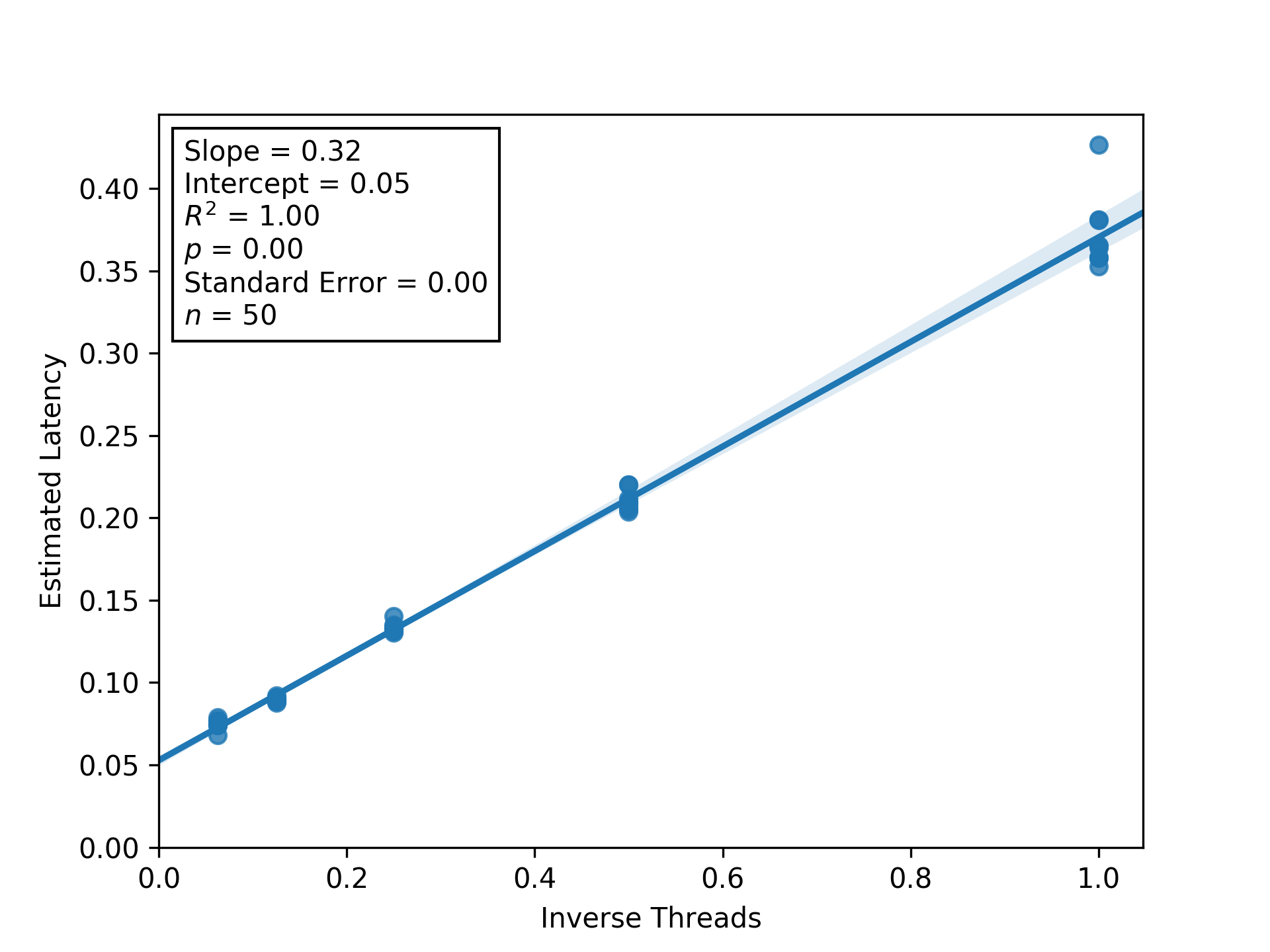 Figure RBITC.
Regression between inverse thread count and estimated latency to estimate threading efficiency and parallel/serial fractions.
Shaded regions are bootstrapped 95% confidence intervals.
Generated via Script DUMFD.
Figure RBITC.
Regression between inverse thread count and estimated latency to estimate threading efficiency and parallel/serial fractions.
Shaded regions are bootstrapped 95% confidence intervals.
Generated via Script DUMFD.
| Parameter | Estimate | Lower Bound | Upper Bound |
|---|---|---|---|
| Parallel Fraction | 0.858 | 0.845 | 0.870 |
| Serial Fraction | 0.142 | 0.130 | 0.155 |
| Threading Efficiency | 0.448 | 0.398 | 0.502 |
| Execution Seconds per Unit Work | 0.370 | 0.358 | 0.383 |
| Latency @ 1 Threads | 0.371 | 0.362 | 0.380 |
| Latency @ 2 Threads | 0.210 | 0.208 | 0.213 |
| Latency @ 4 Threads | 0.133 | 0.132 | 0.135 |
| Latency @ 8 Threads | 0.090 | 0.088 | 0.091 |
| Latency @ 16 Threads | 0.075 | 0.073 | 0.077 |
| Overhead @ 1 Threads | 0.104 | 0.032 | 0.176 |
| Overhead @ 2 Threads | 0.177 | 0.138 | 0.217 |
| Overhead @ 4 Threads | 0.102 | 0.053 | 0.151 |
| Overhead @ 8 Threads | 0.094 | 0.016 | 0.173 |
| Overhead @ 16 Threads | 0.341 | 0.137 | 0.544 |
Table EPUAL. Estimated parameters. Upper and lower bounds indicate \(\geq95\%\) confidence. Generated via Script DUMFD.
🔗 Thread Count 1
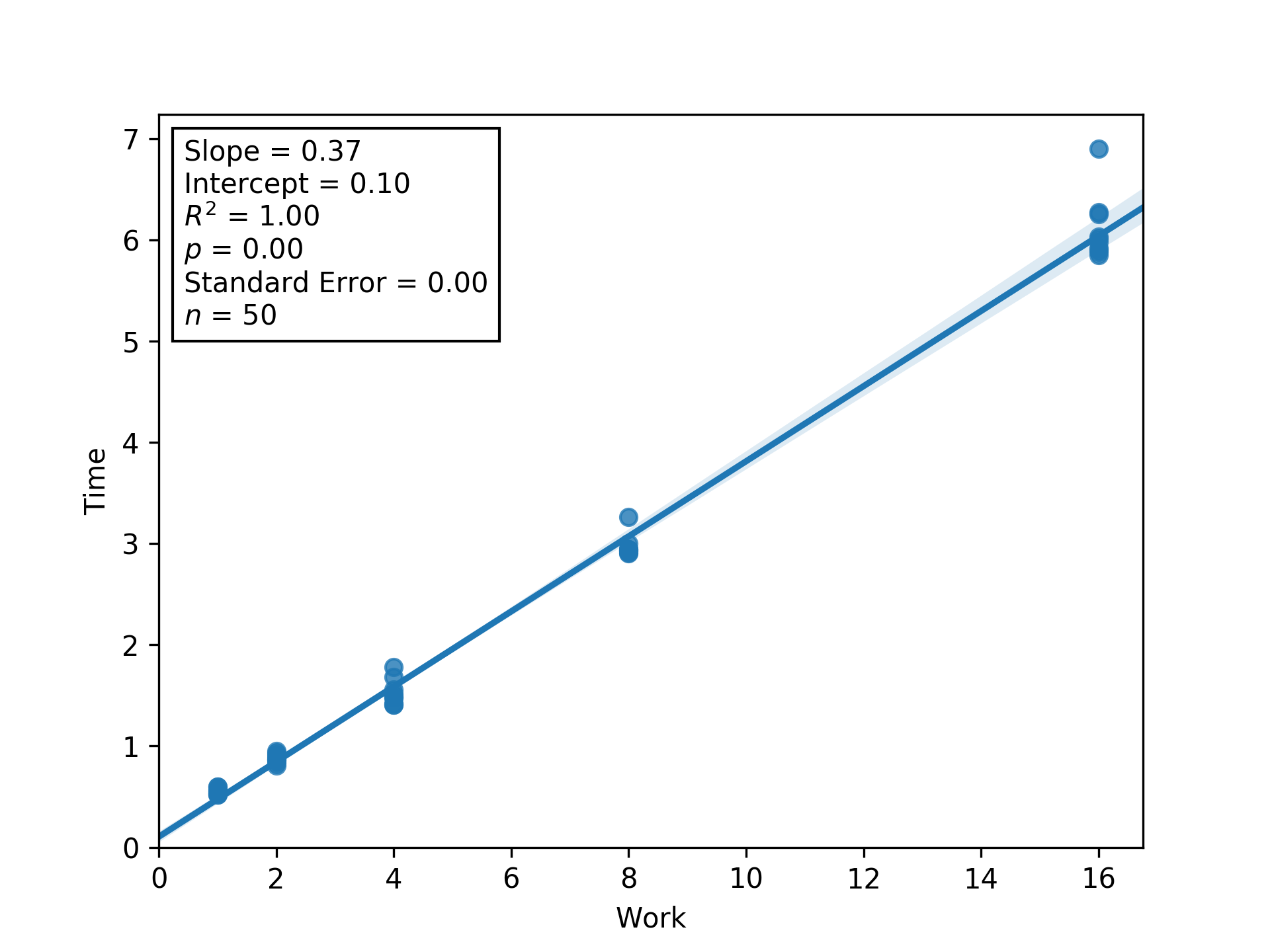 Figure L1RBW.
Regression between work and time (seconds) to estimate latency (i.e., inverse throughput) and overhead at load factor 1.
Shaded regions are bootstrapped 95% confidence intervals.
Generated via Script DUMFD.
Figure L1RBW.
Regression between work and time (seconds) to estimate latency (i.e., inverse throughput) and overhead at load factor 1.
Shaded regions are bootstrapped 95% confidence intervals.
Generated via Script DUMFD.
🔗 Thread Count 2
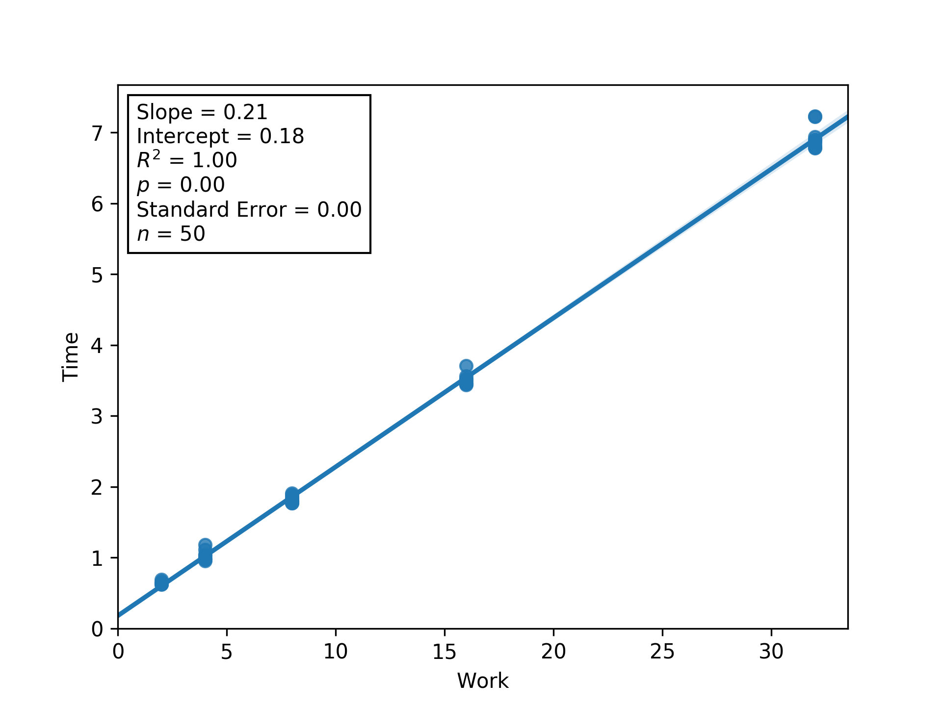 Figure L2RBW.
Regression between work and time (seconds) to estimate latency (i.e., inverse throughput) and overhead at load factor 2.
Shaded regions are bootstrapped 95% confidence intervals.
Generated via Script DUMFD.
Figure L2RBW.
Regression between work and time (seconds) to estimate latency (i.e., inverse throughput) and overhead at load factor 2.
Shaded regions are bootstrapped 95% confidence intervals.
Generated via Script DUMFD.
🔗 Thread Count 4
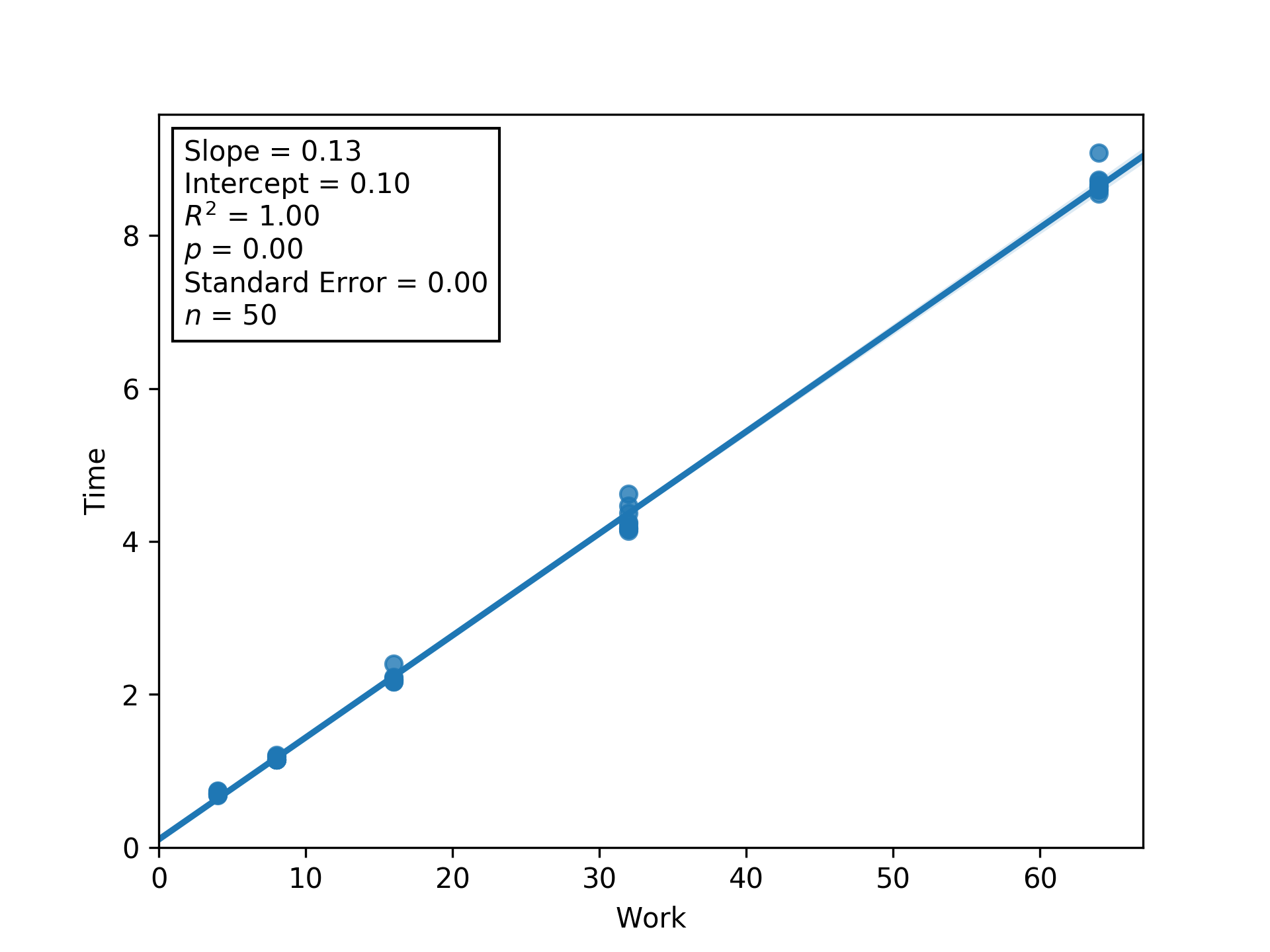 Figure L4RBW.
Regression between work and time (seconds) to estimate latency (i.e., inverse throughput) and overhead at load factor 4.
Shaded regions are bootstrapped 95% confidence intervals.
Generated via Script DUMFD.
Figure L4RBW.
Regression between work and time (seconds) to estimate latency (i.e., inverse throughput) and overhead at load factor 4.
Shaded regions are bootstrapped 95% confidence intervals.
Generated via Script DUMFD.
🔗 Thread Count 8
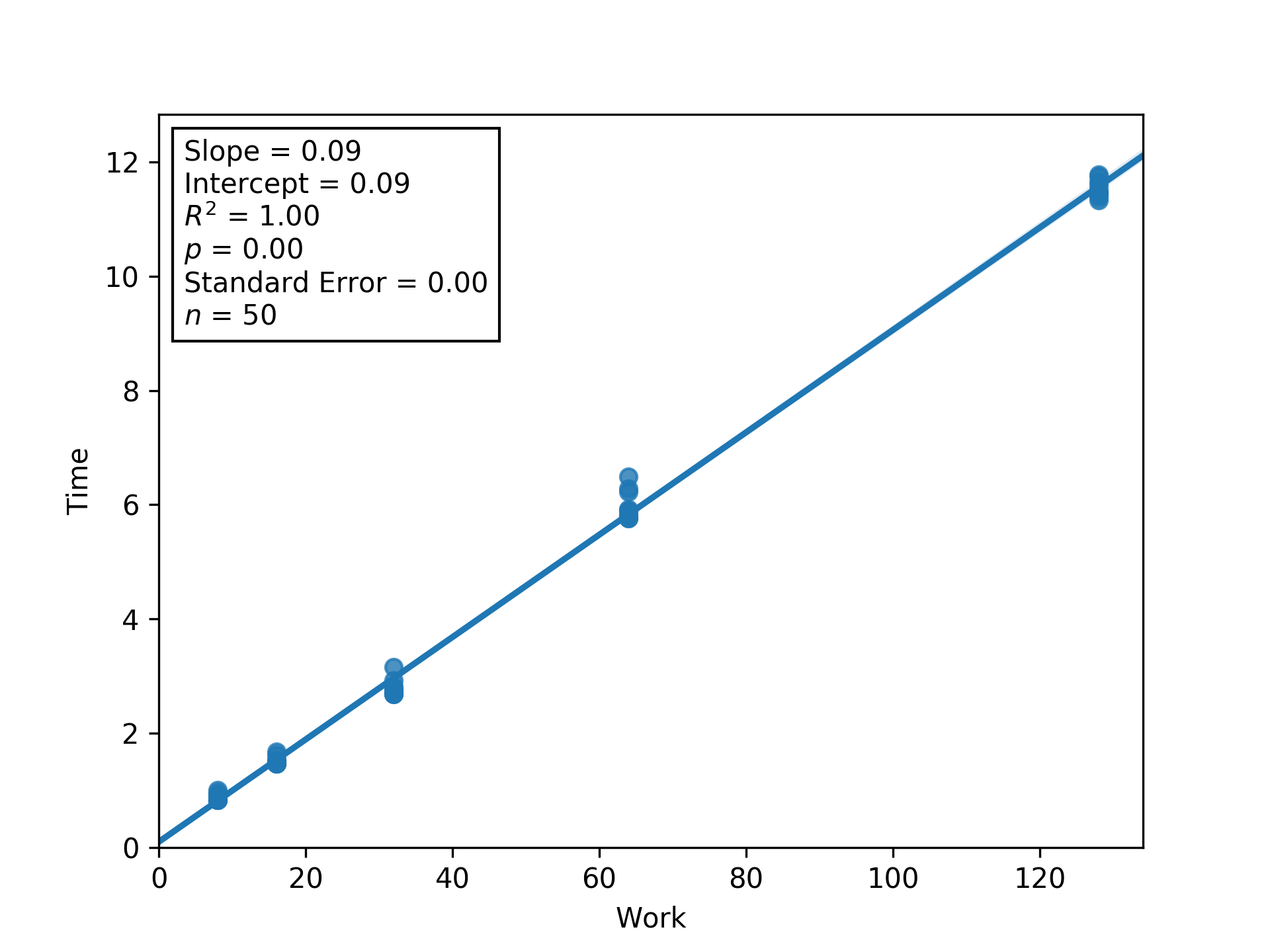 Figure L8RBW.
Regression between work and time (seconds) to estimate latency (i.e., inverse throughput) and overhead at load factor 8.
Shaded regions are bootstrapped 95% confidence intervals.
Generated via Script DUMFD.
Figure L8RBW.
Regression between work and time (seconds) to estimate latency (i.e., inverse throughput) and overhead at load factor 8.
Shaded regions are bootstrapped 95% confidence intervals.
Generated via Script DUMFD.
🔗 Thread Count 16
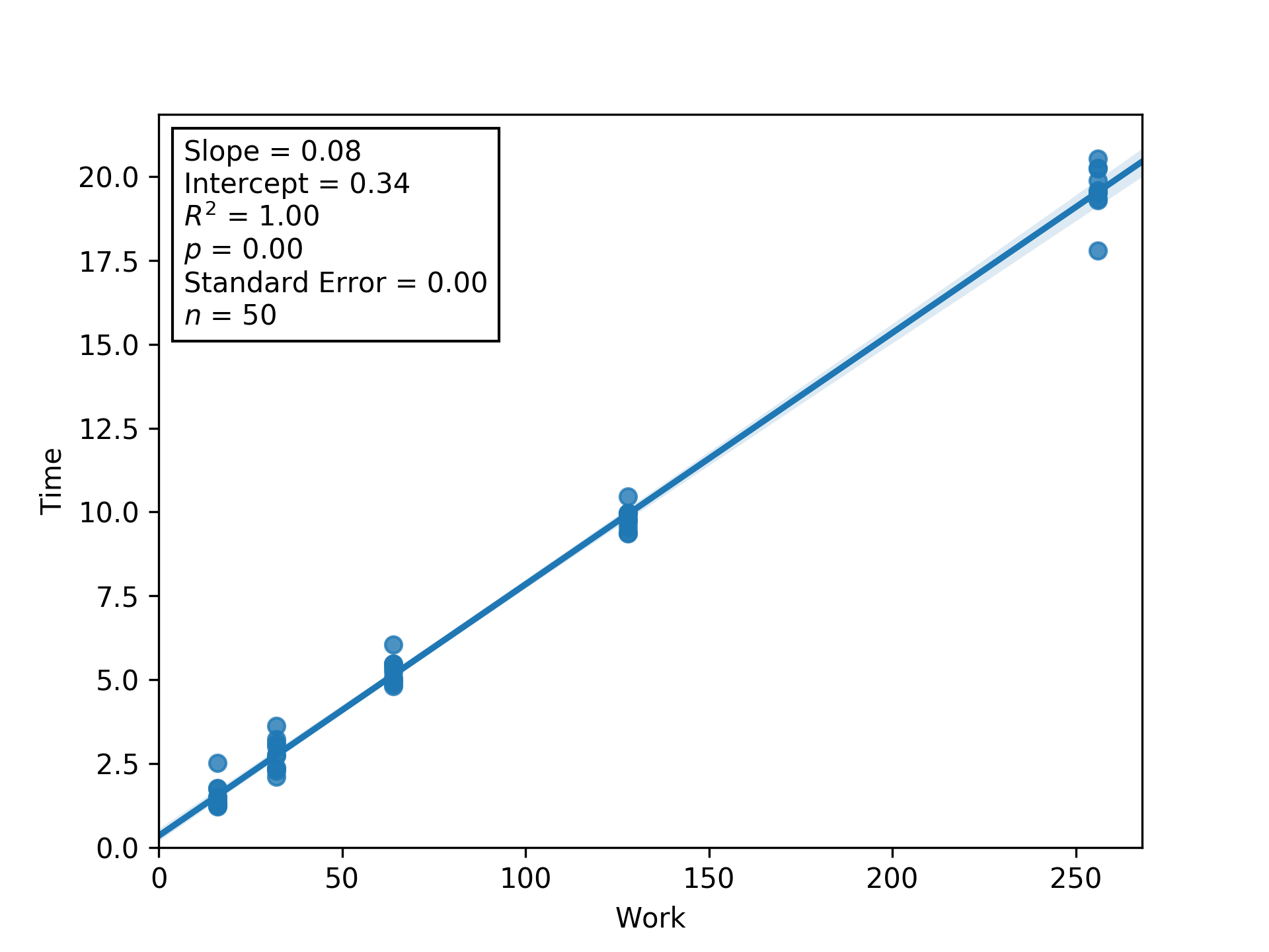 Figure L16IT.
Regression between work and time (seconds) to estimate latency (i.e., inverse throughput) and overhead at load factor 16.
Shaded regions are bootstrapped 95% confidence intervals.
Generated via Script DUMFD.
Figure L16IT.
Regression between work and time (seconds) to estimate latency (i.e., inverse throughput) and overhead at load factor 16.
Shaded regions are bootstrapped 95% confidence intervals.
Generated via Script DUMFD.
🔗 Scripts
OUT_FILE="malloc=mimalloc+ext=.csv"
echo "Threads,Work,Load,Replicate,Time" > $OUT_FILE
for NUM_THREADS in 1 2 4 8 16; do
  for LOAD_PER in 1 2 4 8 16; do
    AMT_WORK=$(( $NUM_THREADS * $LOAD_PER ))
    for REP in {0..9}; do
      echo "NUM_THREADS: ${NUM_THREADS}"
      echo "AMT_WORK: ${AMT_WORK}"
      echo "LOAD_PER: ${LOAD_PER}"
      echo "REP: ${REP}"
      export OMP_NUM_THREADS=$NUM_THREADS
      export DIM=$(bc <<< "sqrt(${AMT_WORK} * 100)")
      echo "DIM: ${DIM}"
      /usr/bin/time -f "%e" -o tmp \
        ./dishtiny -RUN_LENGTH 200 -GRID_W ${DIM} -GRID_H ${DIM} \
        > /dev/null 2>&1
      ELAPSED_TIME=$(cat tmp)
      echo "ELAPSED_TIME: ${ELAPSED_TIME}"
      echo "${NUM_THREADS},${AMT_WORK},${LOAD_PER},${REP},${ELAPSED_TIME}" >> $OUT_FILE
    done;
  done;
done
import pandas as pd
import statsmodels.formula.api as smf
from scipy.stats import stats

import matplotlib.pyplot as plt
from matplotlib.offsetbox import AnchoredText
import seaborn as sns

import itertools as it
import numpy as np
from slugify import slugify
from keyname import keyname as kn
from iterpop import iterpop as ip


def estimate_latency(group):
  '''
  Use a linear regression to estimate time per work from a Pandas GroupBy.
  '''
  model = smf.glm(
    formula='Time ~ Work',
    data=group,
  ).fit()

  # pack up information about parameter estimates
  # so they can be programatically unpacked later
  decoder = {
    'Intercept' : 'Overhead',
    'Work' : 'Latency',
  }

  for spec, val in (
        (
            {
              'statistic' : statistic,
              'name' : decoder[parameter],
            },
            getter(parameter)
        ) for parameter in model.params.keys()
        for statistic, getter in (
          ('Estimated', lambda param: model.params[parameter]),
          ('Lower Bound', lambda param: model.conf_int()[0][param]),
          ('Upper Bound', lambda param: model.conf_int()[1][param]),
         )
    ):
    group['{statistic} {name}'.format(**spec)] = val

  return group

def _do_plot(df, x, y, ax=None):
  '''
  Wrap a call to Seaborn's regplot.
  '''
  res = sns.regplot(
    data=df,
    x=x,
    y=y,
    truncate=False,
    ax=ax
  )
  res.set_xlim(0, )
  res.set_ylim(0, )

  return res


def plot_regression(df, x, y, extra_names={}):
  '''Plot a regression with annotated statistics.'''
  # ugly hack to include origin in plot bounds
  plt.clf()
  ax = _do_plot(df, x, y)
  xlim, ylim = ax.get_xlim(), ax.get_ylim()
  ax.cla()
  ax.set_xlim(*xlim)
  ax.set_ylim(*ylim)
  _do_plot(df, x, y, ax=ax)

  # calculate some regression statistics...
  info = [
    ("{} = " + ("{}" if isinstance(v, int) else "{:.2f}")).format(k, v)
    for k, v in it.chain(zip(
      [
        'Slope',
        'Intercept',
        '$R^2$',
        '$p$',
        'Standard Error',
      ],
      stats.linregress(df[x],df[y]),
    ), [
      ('$n$', len(df))
    ])
  ]

  # ... and annotate regression statistics onto upper left
  at = AnchoredText(
    '\n'.join(info),
    frameon=True,
    loc='upper left',
  )
  ax.add_artist(at)

  # save to file
  # and assert df['Load'] is homogeneous
  plt.savefig(
    kn.pack({**{
      'x' : slugify(x),
      'y' : slugify(y),
      'ext': '.png',
    },**extra_names}),
    transparent=True,
    dpi=300,
  )


def deduce_properties(**kwargs):
  '''
  Deduce scaling properties we're trying to estimate from params computed
  via linear regression between Inverse Threads and Estimated Latency.
  '''
  res = {}

  res['Execution Seconds per Unit Work'] =  (
    kwargs['Intercept'] + kwargs['Q("Inverse Threads")']
  )
  res['Serial Fraction'] = (
    kwargs['Intercept'] / res['Execution Seconds per Unit Work']
  )
  res['Parallel Fraction'] = 1.0 - res['Serial Fraction']
  res['Threading Efficiency'] = (
    res['Serial Fraction'] / kwargs['Q("Inverse Threads")']
  )

  return res

def estimate_properties(model):
  '''
  Calculate estimates and bounds on scaling properties of interest
  from estimates and confidence intervals of params computed
  via linear regression between Inverse Threads and Estimated Latency
  '''
  # from DataFrame...
  #             0     1
  # Parameter1  val1  val2
  # Parameter2  val3  val4
  # ... to dict of lists
  # {
  #   Parameter1 : [val1, val2]
  #   Parameter2 : [val3, val4]
  # }
  conf_ints = {
      col : list(bounds)
      for col, bounds in model.conf_int().iterrows()
  }

  # take the product of dicts
  # use .items() to preserve ordering
  # adapted from http://stephantul.github.io/python/2019/07/20/product-dict/
  #
  # from to dict of lists...
  # {
  #   Parameter1 : [val1, val2]
  #   Parameter2 : [val3, val4]
  # }
  # ... to list of dicts (product of value lists)
  # [
  #   {
  #     Parameter1 : val1,
  #     Parameter2 : val3,
  #   },
  #   {
  #     Parameter1 : val1,
  #     Parameter2 : val4,
  #   },
  #   {
  #     Parameter1 : val2,
  #     Parameter2 : val3,
  #   },
  #   {
  #     Parameter1 : val2,
  #     Parameter2 : val4,
  #   },
  # ]
  keys, values = zip(*conf_ints.items())
  corners = [
    dict(zip(keys, bundle))
    for bundle in it.product(*values)
  ]
  assert(
    len(corners) == np.prod([len(val) for val in conf_ints.values()])
  )

  # from to dict of lists of raw parameter values...
  # [
  #   {
  #     Parameter1 : val1,
  #     Parameter2 : val3,
  #   },
  #   {
  #     Parameter1 : val1,
  #     Parameter2 : val4,
  #   },
  #   etc.
  # ]
  # ... to DataFrame of deduced parameters
  #    Parameter3   Parameter4   Parameter5
  # 0  val          val          val
  # 1  val          val          val
  # etc.
  extremes = pd.DataFrame([
    deduce_properties(**corner)
    for corner in corners
  ])

  # from DataFrame of deduced parameters...
  #    Parameter3   Parameter4   Parameter5
  # 0  val5         val6         val7
  # 1  val8         val9         val10
  # etc.
  # ... to DataFrame of deduced parameter bounds and estimates
  #    Parameter    Lower Bound   Upper Bound   Estimate
  # 0  Parameter3   val           val           val
  # 1  Parameter4   val           val           val
  # 2  Parameter5   val           val
  res = pd.DataFrame([
    {
      'Parameter' : param,
      'Lower Bound' : extremes[param].min(),
      'Upper Bound' : extremes[param].max(),
      'Estimate' : deduce_properties(
        **model.params
      )[param],
    } for param in extremes
  ])

  return res


# load and set up DataFrame
df = pd.read_csv(kn.pack({
  "malloc" : "mimalloc",
  "ext" : ".csv",
}))
df['Inverse Threads'] = 1 / df['Threads']


# independently for each replicate, estimate overhead and latency
df = df.groupby([
  'Threads',
  'Replicate',
]).apply(
  estimate_latency,
)

# model relationship between latency (inverse throughput) and thread count
model = smf.glm(
  formula='Q("Estimated Latency") ~ Q("Inverse Threads")',
  data=df.drop_duplicates([
    'Threads',
    'Replicate',
  ]),
).fit()

# start a dataframe to collect estimates of scaling properties
res = estimate_properties(model)

# visualize regression
plot_regression(
  df.drop_duplicates([
    'Threads',
    'Replicate',
  ]),
  'Inverse Threads',
  'Estimated Latency',
)

# now, for posterity...
# estimate overhead and latency using /all/ replicates
df = df.groupby(
  'Threads',
).apply(
  estimate_latency,
)

# plot regressions used to estimate overhead and latency
for threads, chunk in df.groupby(
  'Threads',
):
  plot_regression(
    chunk,
    'Work',
    'Time',
    extra_names={'threads' : threads},
  )

# extract estimates of overhead and latency
res = res.append(pd.DataFrame([
    {
      'Parameter' : '{} @ {} Threads'.format(name, threads),
      'Lower Bound' : ip.pophomogeneous(chunk['Lower Bound ' + name]),
      'Upper Bound' : ip.pophomogeneous(chunk['Upper Bound ' + name]),
      'Estimate' : ip.pophomogeneous(chunk['Estimated ' + name]),
    } for threads, chunk in df.groupby('Threads')
    for name in ('Overhead', 'Latency')
]))

# consolidate and save computed estimates and bounds
res.sort_values([
  'Parameter',
]).to_csv(
  'parameter_estimates.csv',
  index=False,
)
import pandas as pd
import seaborn as sns
import matplotlib.pyplot as plt
from keyname import keyname as kn
from iterpop import iterpop as ip

# load and set up DataFrame
actual = pd.read_csv(kn.pack({
  "malloc" : "mimalloc",
  "ext" : ".csv",
}))
actual["Type"] = "Actual"

# get ready to calculate ideal timings in terms actual timings
# with thread count 1
ideal = actual.copy()
ideal["Type"] = "Ideal"

# helper functions
get_baseline_idx = lambda row: actual[
    (actual["Work"] == row["Work"])
    & (actual["Replicate"] == row["Replicate"])
]["Threads"].idxmin()

get_baseline_time = lambda row: actual.iloc[
    get_baseline_idx(row)
]["Time"]

get_baseline_threads = lambda row: actual.iloc[
    get_baseline_idx(row)
]["Threads"]

# calculate ideal time in terms of lowest-threaded observation
ideal["Time"] = ideal.apply(
    lambda row: (
        get_baseline_time(row)
        * get_baseline_threads(row)
        / row["Threads"]
    ),
    axis=1,
)

# drop thread counts from ideal that were defined identically to actual
ideal = ideal.drop(ideal.index[
    ideal.apply(
        lambda row: row["Threads"] == ideal[
            ideal["Work"] == row["Work"]
        ]["Threads"].min(),
        axis=1,
    ),
])

# merge in newly-calculated ideal timings
df = pd.concat([ideal, actual])

# draw plot
g = sns.FacetGrid(
  df,
  col="Work",
  col_wrap=3,
  margin_titles="true",
  sharey=False,
)

g.map(
  sns.barplot,
  "Threads",
  "Time",
  "Type",
  hue_order=sorted(df["Type"].unique()),
  order=sorted(df["Threads"].unique()),
  palette=sns.color_palette(),
).add_legend()

plt.savefig(
  "dishtiny-profile-work-summary.png",
  transparent=True,
  dpi=300,
)
import pandas as pd
import seaborn as sns
import matplotlib.pyplot as plt
from keyname import keyname as kn

# load and set up DataFrame
actual = pd.read_csv(kn.pack({
  "malloc" : "mimalloc",
  "ext" : ".csv",
}))
actual["Type"] = "Actual"

# get ready to calculate ideal timings in terms actual timings
# with thread count 1
ideal = actual.copy()
ideal["Type"] = "Ideal"

# helper functions
get_baseline_idx = lambda row: actual[
    (actual["Load"] == row["Load"])
    & (actual["Replicate"] == row["Replicate"])
]["Threads"].idxmin()

get_baseline_time = lambda row: actual.iloc[
    get_baseline_idx(row)
]["Time"]

# calculate ideal time in terms of lowest-threaded observation
ideal["Time"] = ideal.apply(
    lambda row: get_baseline_time(row),
    axis=1,
)

# drop thread counts from ideal that were defined identically to actual
ideal = ideal.drop(ideal.index[
    ideal.apply(
        lambda row: row["Threads"] == ideal[
            ideal["Load"] == row["Load"]
        ]["Threads"].min(),
        axis=1,
    ),
])

# merge in newly-calculated ideal timings
df = pd.concat([ideal, actual])

# draw plot
g = sns.FacetGrid(
  df,
  col="Load",
  col_wrap=3,
  margin_titles="true",
  sharey=False,
)

g.map(
  sns.barplot,
  "Threads",
  "Time",
  "Type",
  hue_order=sorted(df["Type"].unique()),
  order=sorted(df["Threads"].unique()),
  palette=sns.color_palette(),
).add_legend()

plt.savefig(
  "dishtiny-profile-load-summary.png",
  transparent=True,
  dpi=300,
)