Practical Steps Toward Indefinite Scalability: In Pursuit of Robust Computational Substrates for Open-Ended Evolution
contents
- Abstract
- Introduction
- Methods
- Case Study: Interconnect Resource Sharing
- Case Study: Interconnect Messaging
- Wiring a Generic Small World Graph
- Wiring an Ideal Space-Filling Hierarchical Tree without Log-Time Physical Interconnects
- Wiring an Ideal Space-Filling Hierarchical Tree with Log-Time Physical Interconnects
- Wiring a Watts-Strogatz Graph
- Conclusion
- Let’s Chat
- Cite This Post
- Footnotes
- References
- Acknowledgements
🔗 Abstract
Studying how artificial evolutionary systems can continually produce novel artifacts of increasing complexity has proven to be a rich vein for practical, scientific, philosophical, and artistic innovations. Unfortunately, existing computational artificial life systems appear constrained by practical limitations on simulation scale. The concept of indefinite scalability describes constraints on open-ended systems necessary to incorporate theoretically unbounded computational resources. Here, we argue that along the path to indefinite scalability, we must consider practical scalability: how can we design open-ended evolutionary systems that make effective use of existing, commercially-available distributed-computing hardware? We highlight log-time hardware interconnects as a potentially fruitful tool for practical scalability and describe how digital evolution systems might be constructed to exploit physical log-time interconnects. We extend the DISHTINY digital multicellularity framework to allow cells to establish long-distance cell-cell interconnects that, in implementation, could take advantage of log-time physical interconnects. We examine two case studies of evolved strains, demonstrating how evolved cells adaptively exploit these interconnects.
🔗 Introduction
The challenge, and promise, of open-ended evolution has animated decades of inquiry and discussion within the artificial life community [Packard et al., 2019]. The difficulty of devising models that produce characteristic outcomes of open-ended evolution suggests profound philosophical or scientific blind spots in our understanding of the natural processes that gave rise to contemporary organisms and ecosystems. Already, pursuit of open-ended evolution has yielded paradigm-shifting insights. For example, novelty search demonstrated how processes promoting non-adaptive diversification can ultimately yield adaptive outcomes that were previously unattainable [Lehman and Stanley, 2011]. Such work lends insight to fundamental questions in evolutionary biology, such as the relevance — or irrelevance – of natural selection with respect to increases in complexity [Lehman, 2012; Lynch, 2007] and the origins of evolvability [Lehman and Stanley, 2013; Kirschner and Gerhart, 1998]. Evolutionary algorithms devised in support of open-ended evolution models also promise to deliver tangible broader impacts on society. Possibilities include the generative design of engineering solutions, consumer products, art, video games, and AI systems [Nguyen et al., 2015; Stanley et al., 2017].
Preceding decades have witnessed advances toward defining — quantitatively and philosophically — the concept of open-ended evolution [Lehman and Stanley, 2012; Dolson et al., 2019; Bedau et al., 1998] as well as investigating causal phenomena that promote open-ended dynamics such as ecological dynamics, selection, and evolvability [Dolson, 2019; Soros and Stanley, 2014; Huizinga et al., 2018]. Together, methodological and theoretical advances have begun to yield evidence that the generative potential of artificial life systems is — at least in part — meaningfully constrained by available compute resources [Channon, 2019].
🔗 Advances in Modern Compute Resources Rely on Distribution and Parallelism
Since the turn of the century, advances in the clock speed of traditional serial processors have trailed off [Sutter, 2005]. Existing technologies have begun to encounter fundamental constraints including power use and thermal dissipation [Markov, 2014]. Instead, hardware innovation began to revolve around multiprocessing [Hennessy and Patterson, 2011, p.55] and hardware acceleration (e.g., GPU, FPGA, etc.) [Che et al., 2008]. For scientific and engineering applications, individual multiprocessors and accelerators are joined together with fast interconnects to yield so-called high-performance computing clusters [Hennessy and Patterson, 2011, p.436]. Until fundamental changes to computing technology transpire, scaling up artificial life compute power will require taking advantage of these existing parallel and distributed systems.
🔗 Distributed Hardware in Digital Evolution
Digital evolution practitioners have a rich history of leveraging distributed hardware. It is common practice to distribute multiple self-isolated instantiations of evolutionary runs over multiple hardware units. In scientific contexts, this practice yields replicate datasets that provide statistical power to answer research questions [Dolson and Ofria, 2017]. In applied contexts, this practice yields many converged populations that can be scavenged for the best solutions overall [Hornby et al., 2006].
Another established practice is to use “island models” where individuals are transplanted between populations that are otherwise independently evolving across distributed hardware. Koza and collaborators’ genetic programming work with a 1,000-cpu Beowulf cluster typifies this approach [Bennett III et al., 1999].
In recent years, Sentient Technologies spearheaded digital evolution projects on an unprecedented computational scale, comprising over a million CPUs and capable of a peak performance of 9 petaflops [Miikkulainen et al., 2019]. According to its proponents, the scale and scalability of this DarkCycle system was a key aspect of its conceptualization [Gilbert, 2015]. Much of the assembled infrastructure was pieced together from heterogeneous providers and employed on a time-available basis [Blondeau et al., 2012]. Unlike island models where selection events are performed independently on each CPU, this scheme transferred evaluation criteria between computational instances (in addition to individual genomes) [Hodjat and Shahrzad, 2013].
Sentient Technologies also accelerated the deep learning training process by using many massively-parallel hardware accelerators (e.g., 100 GPUs) to evaluate the performance of candidate neural network architectures on image classification, language modeling, and image captioning problems [Miikkulainen et al., 2019]. Analogous work parallelizing the evaluation of an evolutionary individual over multiple test cases in the context of genetic programming has used GPU hardware and vectorized CPU operations [Harding and Banzhaf, 2007b; Langdon and Banzhaf, 2019].
Existing applications of concurrent approaches to digital evolution distribute populations or individuals across hardware to process them with minimal interaction. Task independence facilitates this simple, efficient implementation strategy, but precludes application on elements that are not independent. Parallelizing evaluation of a single individual often emphasizes data-parallelism over independent test cases, which are subsequently consolidated into a single fitness profile. With respect to model parallelism, Harding has notably applied GPU acceleration to cellular automata models of artificial development systems, which involve intensive interaction between spatially-distributed instantiation of a genetic program [Harding and Banzhaf, 2007a]. However, in systems where evolutionary individuals themselves are parallelized they are typically completely isolated from each other.
We argue that, in a manner explicitly accommodating capabilities and limitations of available hardware, open-ended evolution should prioritize dynamic interactions between simulation elements situated across physically distributed hardware components.
🔗 Leveraging Distributed Hardware for Open-Ended Evolution
Unlike most existing applications of distributed computing in digital evolution, open-ended evolution researchers should prioritize dynamic interactions among distributed simulation elements. Parallel and distributed computing enables larger populations and metapopulations. However, ecologies, co-evolutionary dynamics, and social behavior all necessitate dynamic interactions among individuals.
Distributed computing should also enable more computationally intensive or complex individuals. Developmental processes and emergent functionality necessitate dynamic interactions among components of an evolving individual. Even at a scale where individuals remain computationally tractable on a single hardware component, modeling them as a collection of discrete components configured through generative development (i.e., with indirect genetic representation) can promote scalable properties [Lipson, 2007] such as modularity, regularity, and hierarchy [Hornby, 2005; Clune et al., 2011]. Developmental processes may also promote canalization [Stanley and Miikkulainen, 2003], for example through exploratory processes and compensatory adjustments [Gerhart and Kirschner, 2007]. To reach this goal, David Ackley has envisioned an ambitious design for modular distributed hardware at a theoretically unlimited scale [Ackley and Cannon, 2011] and demonstrated an algorithmic substrate for emergent agents that can take advantage of it [Ackley, 2018].
🔗 A Path of Expanding Computational Scale
While by no means certain, the idea that orders-of-magnitude increases in compute power will open up qualitatively different possibilities with respect to open-ended evolution is well founded. Spectacular advances achieved with artificial neural networks over the last decade illuminate a possible path toward this outcome. As with digital evolution, artificial neural networks (ANNs) were traditionally understood as a versatile, but auxiliary methodology — both techniques were described as “the second best way to do almost anything” [Miaoulis and Plemenos, 2008; Eiben, 2015]. However, the utility and ubiquity of ANNs has since increased dramatically. The development of AlexNet is widely considered pivotal to this transformation. AlexNet united methodological innovations from the field (such as big datasets, dropout, and ReLU) with GPU computing that enabled training of orders-of-magnitude-larger networks. In fact, some aspects of their deep learning architecture were expressly modified to accommodate multi-GPU training [Krizhevsky et al., 2012]. By adapting existing methodology to exploit commercially available hardware, AlexNet spurred the greater availability of compute resources to the research domain and eventually the introduction of custom hardware to expressly support deep learning [Jouppi et al., 2017].
Similarly, progress toward realizing artificial life systems with indefinite scalability seems likely to unfold as incremental achievements that spur additional interest and resources in a positive feedback loop with the development of methodology, software, and eventually specialized hardware to take advantage of those resources. In addition to developing hardware-agnostic theory and methodology, we believe that pushing the envelope of open-ended evolution will analogously require designing systems that leverage existing commercially-available parallel and distributed compute resources at circumstantially-feasible scales. Modern high-performance scientific computing clusters appear perhaps the best target to start down this path. These systems combine memory-sharing parallel architectures comprising dozens of cores (commonly targeted using OpenMP [Dagum and Menon, 1998] and low-latency high-throughput message-passing between distributed nodes (commonly targeted using MPI [Clarke et al., 1994]).
Contemporary scientific computing clusters lack key characteristics required for indefinite scalability: fault tolerance and arbitrary extensibility. However, they also may offer an opportunity not available in an indefinitely scalable framework: log-time interconnects [Mollah et al., 2018].
🔗 Instantiating Small-World Networks on Parallel and Distributed Hardware
Many natural systems — such as ecosystems, genetic regulatory networks, and neural networks — are known to exhibit small-world patterns of connectivity or interaction among components [Bassett and Bullmore, 2017; Fox and Bellwood, 2014; Gaiteri et al., 2014]. In small-world graphs, mean path length (the number of edges traversed on a shortest-route) between arbitrary components scales logarithmically with system size [Watts and Strogatz, 1998]. We anticipate that open-ended phenomena emerging across distributed hardware might also involve small-world connectivity dynamics.
What would the impact be of providing a system of hierarchical log-time hardware interconnects as opposed to relying solely on local hardware interconnects?
In Sections WAGSW, WAISO, WAISW, and WAWSG, we analyze the scaling relationship between system size and expected node-to-node hops traversed between computational elements interacting as part of an emergent small-world network. [Footnote WDWCM]
- with and without hierarchical log-time physical interconnects between computational nodes, and
- with computational nodes embedded on one-, two-, or three-dimensional computational meshes.
In Section WAGSW, we find that expected hops over edges weighted by edge betweenness centrality scales polynomially in all cases without hierarchical physical interconnects. With hierarchical physical interconnects, a logarithmic scaling relationship can be achieved.
In Sections WAISO, WAISW we find that hierarchical physical interconnects yield better best-case mean hops per edge in the case of a one-dimensional computational mesh. Interestingly, asymptotically better outcomes in two- and three- dimensional meshes cannot be guaranteed by hierarchical physical interconnects. This suggests that — even at truly vast scales — emergent inter-component interaction networks could arise with bounded per-hardware-component messaging load.
In Section WAWSG we show that, with a specific traditional construction of small-world graphs, best-case mean hops per edge scales polynomially with graph size. With hierarchical physical interconnects, a logarithmic scaling relationship can still be achieved.
These theoretical analyses suggest that whether log-time physical interconnects deliver asymptotically better mean connection latency and hop-efficiency depend on the structure of the network overlaid on a spatially-distributed hardware system. Although we focus on asymptotic analyses, better scaling coefficients might be achieved with long-distance hardware interconnects. Equivalent asymptotic behavior does not preclude important considerations with respect to performance.
🔗 Exploiting Log-Time Physical Interconnects: a Case Study
What could an artificial life system that exploits log-time hardware interconnects look like?
We present an extension to the DISHTINY platform for studying evolutionary transitions in individuality [Moreno and Ofria, 2019]. In previous work with the system, cells situated on a two-dimensional grid interact exclusively with immediate neighbors. This extension introduces genetic programs that can explicitly-register direct interconnects between (potentially distant) cells for messaging and resource-sharing. Cells establish these interconnects through a genetically-mediated exploratory growth process.
We report a case study of an evolved strain that adaptively employs interconnects to communicate and selectively distribute resources to the periphery of a multicellular organism. In Section CSIM, we report another case study of an evolved strain that adaptively employs over-interconnect messaging to selectively suppress somatic cell reproduction.
In future implementations, explicitly-registered cell-cell interconnects may use log-time physical interconnects. Our prototype implementation exploits shared-memory thread-level parallelism on a single multiprocessor.
🔗 Abstraction, Engineering, and Computational Scale
Although designed with an eye toward scalability, largely along the lines outlined by Ackley, DISHTINY exchanges a uniform, evolutionary-passive substrate for manually-engineered self-replicating cells. Evolutionary transitions in individuality provide a framework to unite self-replicators and induce meaningful functional synthesis of programmatic components tied to individual compute elements. This approach mirrors the philosophy of practicality and feasibility laid out by Channon [Channon, 2019]:
It is not computationally feasible (even if we knew how) for an OEE simulation to start from a sparse fog of hydrogen and helium and transition to a biological-level era, so it is clearly necessary to skip over or engineer in at least some complex features that arose through major transitions in our universe.
DISHTINY engineers-in some complex features (e.g., cellular structure, genetic transmission of variation, explicitly-registered cell-cell interconnects) in a manner that aims to reflect underlying hardware capabilities (e.g., procedural expression of programs, log-time physical interconnects) so they can be fully utilized.
More granular, less prescriptional approaches seem likely to become preferred when orders of magnitude of more compute power — toward the extent envisioned by Ackley — become available. Such systems will address important questions in their own right about the computational foundations of physical and biological reality. Current work developing those systems sets the stage for that eventuality [Ackley, 2018].
🔗 Methods
Our evolutionary case studies employ an extension to the DISHTINY framework for studying fraternal transitions in individuality. Initial work with this system characterized selective pressures for cooperation with kin [Moreno and Ofria, 2019]. We have since extended the system to use the SignalGP event-driven genetic programming technique [Lalejini and Ofria, 2018] to control cell behaviors. Diverse multicellular life histories evolved in SignalGP-enabled DISHTINY evolutionary trials, involving reproductive division of labor, resource sharing (including, in some treatments, endowment of offspring groups), asymmetrical within-group and inter-group phenomena mediated by cell-cell messaging, morphological patterning, gene-regulation mediated life cycles, and adaptive apoptosis [Moreno and Ofria, prep].
DISHTINY simulates individual cells, each of which occupies a tile on a toroidal grid. Cells can reproduce, placing daughter cells into adjoining tiles. We allow cells the opportunity to engage with kin in a cooperative resource-collection task (Supplementary Section A), which can increase their individual cellular reproduction rates [Moreno and Ofria, 2020]. Kin groups are explicitly registered: on birth, a cell is either added to its parent’s group or expelled to establish a new group (Supplementary Section B) [Moreno and Ofria, 2020].
Cells can differentiate between neighbors that are members of their kin group and neighbors that are not and alter their behavior accordingly. Each cell contains four SignalGP instances (all executing the same genetic program), one of which controls cell behavior with respect to each neighbor. These instances may communicate with one another by means of intracellular messaging. In this work, we add a fifth SignalGP instance to the DISHTINY cell. This instance can execute special instructions to establish long-distance interconnects with other cells and engage in resource-sharing and/or message passing with those cells. Figure AOSHW summarizes how SignalGP hardware is arranged within DISHTINY cells.
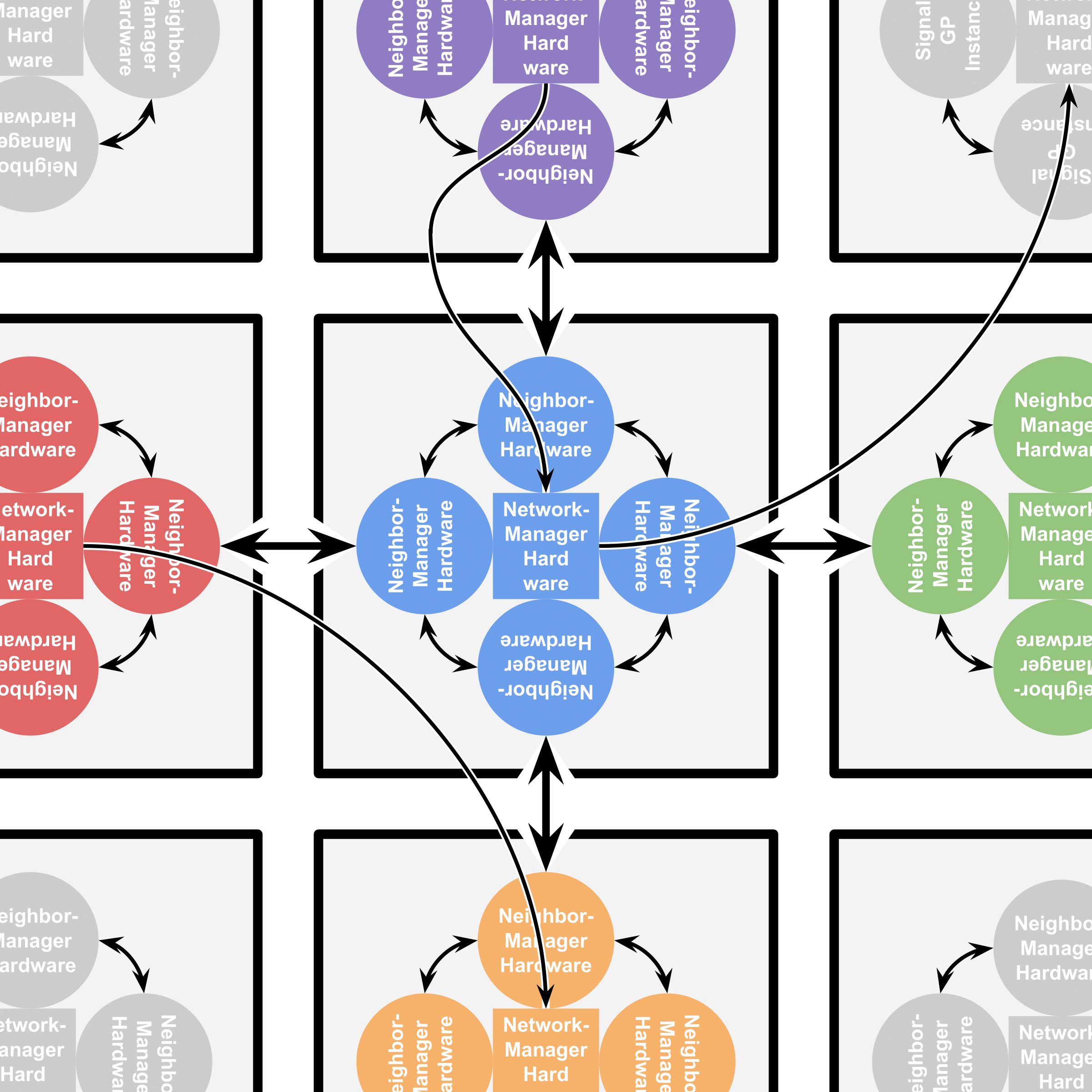 Figure AOSHW:
Arrangement of SignalGP hardware within DISHTINY cells (gray squares).
Neighbor-managing hardware (circles) receive stimuli and control cell behavior with respect to a particular cell neighbor.
Network-managing hardware (interior squares) receive stimuli and control cell
behavior with respect to more distant neighbors a cell has established interconnects with.
Figure AOSHW:
Arrangement of SignalGP hardware within DISHTINY cells (gray squares).
Neighbor-managing hardware (circles) receive stimuli and control cell behavior with respect to a particular cell neighbor.
Network-managing hardware (interior squares) receive stimuli and control cell
behavior with respect to more distant neighbors a cell has established interconnects with.
Long-distance interconnects are established through a developmental process, summarized in Figure IOTDP. The process begins with the placement of two independent search prongs at the originating cell. Each prong performs a random walk over the originating cell’s kin group, accumulating positive or negative feedback based on tags expressed by underfoot cells. If a prong accumulates positive feedback too slowly, it is reset to the location of the better-scoring prong. Once a positive feedback threshold has been reached, the best-scoring prong develops into a full-fledged connection. At this point, the originating cell can begin exchanging messages and/or resource over the connection. Established interconnects may be subsequently removed by either participating cell.
Full details on hardware-level instructions and event-driven environmental cues available to cells are provided in Supplementary Sections D, E, F, and G [Moreno and Ofria, 2020].
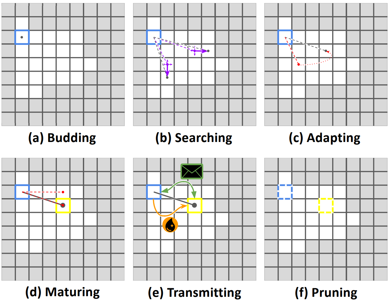 Figure IOTDP:
Illustration of the developmental process used to establish long-distance interconnects.
Cells start by budding developmental search prongs (a) that perform a random search (b), reverting to the most successful search (c) where it matures to establish a connection (d).
Messages and resources can be transmitted over a connection (e) until either cell decides to terminate the connection (f). You can see this developmental process in action in an evolved strain at
Figure IOTDP:
Illustration of the developmental process used to establish long-distance interconnects.
Cells start by budding developmental search prongs (a) that perform a random search (b), reverting to the most successful search (c) where it matures to establish a connection (d).
Messages and resources can be transmitted over a connection (e) until either cell decides to terminate the connection (f). You can see this developmental process in action in an evolved strain at https://mmore500.com/hopto/ap.
🔗 Evolutionary Screens
Our evolutionary screens consisted of 64 independent evolutionary batches. We processed each batch in four-hour epochs to enable efficient job scheduling. Each batch consisted of four isolated 45-by-45 toroidal subpopulations. Subpopulations were completely intermixed in between four-hour steps. To facilitate evolutionary search, in addition to a base mutation rate applied to cell division, additional mutations were applied to cells seeding a toroidal grid at the outset of an epoch or budding to form new kin groups during an epoch.
We screened across four-hour checkpoints of replicate batches to see if messages or resource were being sent over interconnects. We sampled from these populations, performing screens for knockouts of over-interconnect messaging or resource sharing. We then performed a secondary screen on strains with adaptive over-interconnect messaging or resource sharing to determine if re-routing either messages or shared resources decreased fitness.
We measured relative fitness using competition experiments between strains. For some competition experiments reported in the case studies, we provide hyperlinks to load an in-browser DISHTINY simulation with the actual strains that were used. In this web viewer, wild-type strains carry phylogenetic root ID 1 and knockout strains carry ID 2.
🔗 Implementation
We implemented our experimental system using the Empirical library for scientific software development in C++, available at https://github.com/devosoft/Empirical [Ofria et al., 2019].
We used OpenMP to parallelize our main evolutionary replicates, distributing work over two threads.
The code used to perform and analyze our experiments, our figures, data from our experiments, and a live in-browser demo of our system is available via the Open Science Framework at https://osf.io/53vgh/ [Foster and Deardorff, 2017].
🔗 Case Study: Interconnect Resource Sharing
 (a) Hypothesized resource-recruiting mechanism
 (b) Kin groups
 (c) Established interconnects
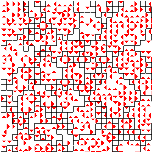
 (d) Spatial distribution of resource-sending cells
 (e) Spatial distribution of resource-receiving cells
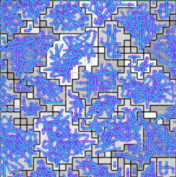
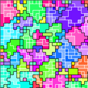
Figure B42CS:
Batch 42 case study overview.
Figures 3b through 3e are generated from a snapshot of a wild-type strain monoculture population.
In these images, each grid tile represents an individual cell.
Cells are organized into kin groups, color-coded by hue in Figure B42CS(b).
Established interconnects are overlaid in blue on Figure B42CS(c).
In Figures B42CS(d) and B42CS(e), kin groups are outlined in black.
Figure B42CS(d) highlights cells that are sending resource over-interconnect.
Figure B42CS(e) highlights cells that are receiving resource over-interconnect.
You can view an animation of the wild-type monoculture at https://mmore500.com/hopto/ao.
This case study was drawn from epoch 24 of batch 42 of the initial set of evolutionary runs.
We initially considered it for further study due to the presence of widespread over-interconnect resource sharing.
After preliminary knockout experiments confirmed the adaptive significance of both over-interconnect resource-sharing and over-interconnect messaging, we set aside the strain for a case study.
The evolutionary history preceding this case study consumed approximately 96 hours of wall-clock time and 736 compute-core hours.
Approximately 30 million simulation updates and 40,000 cellular generations elapsed.
You can view the strain this case study characterizes in a live in-browser simulation at https://mmore500.com/hopto/8.
Our first step was to evaluate whether the intercellular nature of over-interconnect messaging and resource sharing contributed to this strain’s fitness. (It is possible that messaging and/or resource sharing behaviors might generate stimuli on the recipient or side-effects on the sender that have adaptive consequences whether or not the sender and recipient are distinct cells; in such a scenario, cells would be just as well off sending messages and/or resource to themselves.) We performed several competition experiments between the wild-type strain and variants where interconnect messaging and resource sharing was altered to be intracellular instead of intercellular. At the end of competition experiments, we evaluated the relative abundances of wild-type and variant strains. In the first variant strain we tested, all outgoing over-interconnect messages were instead delivered to the sending cell. In 16 out of 16 one-hour competition runs that were seeded half-and-half with the wild-type and variant strains, the wild-type strain drove the variant strain to extinction (one-tailed binomial test; \(p < 0.0001\); 290 S.D 17 cell gens elapsed). We observed a similar outcome with a second variant strain where all outgoing over-interconnect resource sharing was rerouted back to the sending cell (14/16 variant strain extinctions; 16/16 wild-type prevalence; 289 S.D. 25 cell gens elapsed). Finally, a third variant strain where both over-interconnect messaging and over-interconnect resource sharing were returned to the sending cell exhibited the same outcome (16/16 variant strain extinctions; 300 S.D. 23 cell gens elapsed). The intercellular natures of both over-interconnect messaging and resource sharing appear essential to fitness.
Next, we took a closer look at the evolved cellular mechanisms controlling over-interconnect messaging and resource sharing. We monitored hardware execution of the wild-type strain in a monoculture population to detect which signals, messages, and fork/call instructions activated each SignalGP module. We manually cross-referenced this information with a human-readable printout of the strain’s genetic program to construct a hypothesized mechanism shown in Figure B42CS. We hypothesize that cells at the periphery of a registered kin group send messages backwards over incoming interconnects that induce interconnect-originating cells to send them resource. Such a mechanism could preferentially increase resource availability at the group periphery, a region where cell-cell conflict is likely elevated.
We performed a series of four-hour competition experiments between wild type and knockout strains to confirm the adaptive significance of each component of this mechanism.
We began by re-routing stimulus 19, which alerts cells to neighbors that are members of a foreign kin group, to activate a known no-op module.
This knockout strain experienced decreased fitness compared to the wild-type strain (16/16 knockout strain extinctions; one-tailed binomial test; \(p < 0.0001\); 1996 S.D. 280 cell gens elapsed; https://mmore500.com/hopto/ak).
Next, we replaced the over-interconnect messaging instruction that triggers over-interconnect resource-sharing with a no-op instruction.
This knockout strain also experienced decreased fitness (16/16 knockout strain extinctions; 1932 S.D. 223 cell gens elapsed; https://mmore500.com/hopto/al).
We then replaced all eight copies of the over-interconnect resource-sharing instruction triggered by the over-interconnect messaging with no-op instructions, once more yielding a strain with diminished fitness (16/16 knockout strain extinctions; 1860 S.D. 370 cell gens elapsed; https://mmore500.com/hopto/am).
Finally, we confirmed the soundness of our fitness competition methodology by running control wild-type versus wild-type competitions.
As expected, we observed no effect of strain ID on competition dominance (8/16 knockout strain extinctions; 8/16 wild-type strain extinctions; one-tailed binomial test; \(p = 0.60\); 1738 S.D. 217 cell gens elapsed; https://mmore500.com/hopto/aj).
🔗 Case Study: Interconnect Messaging
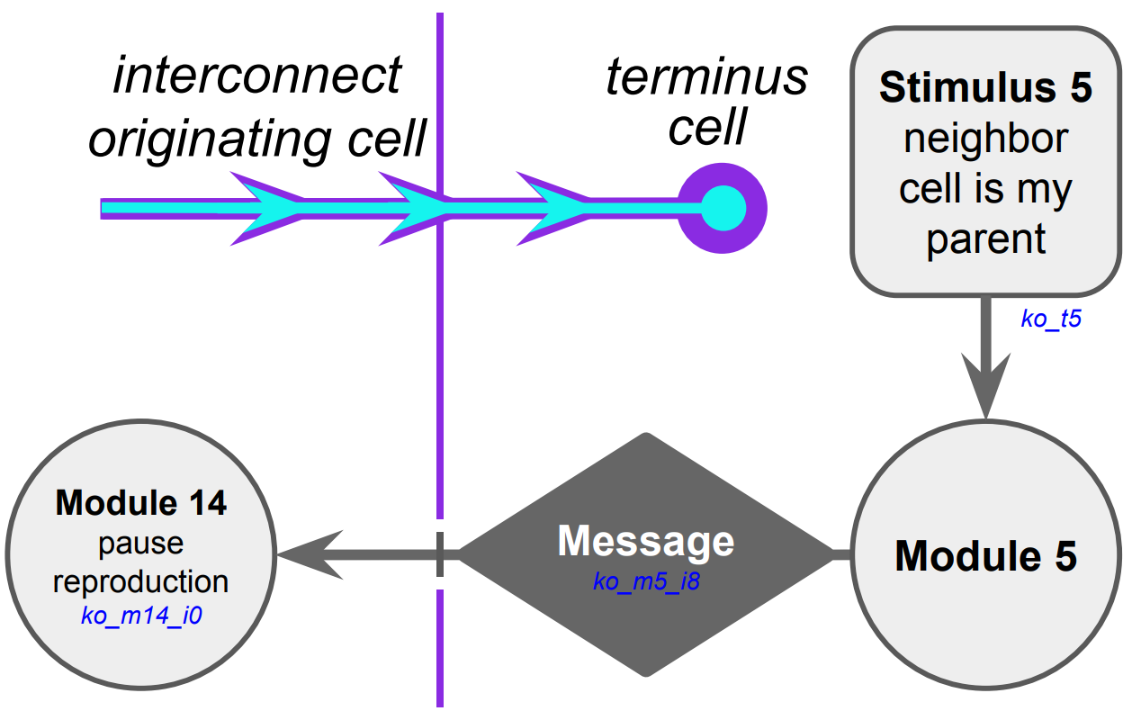 (a) Hypothesized selective reproduction pausing mechanism
 (b) Kin groups
 (c) Established interconnects
 (d) Spatial distribution of stimulus 5
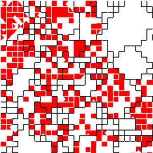 (e) Spatial distribution of module 14 execution
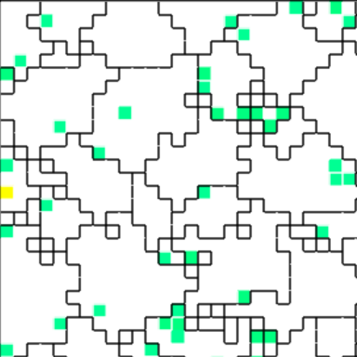
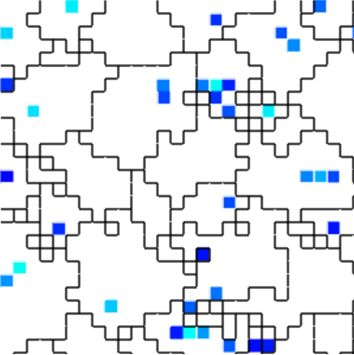
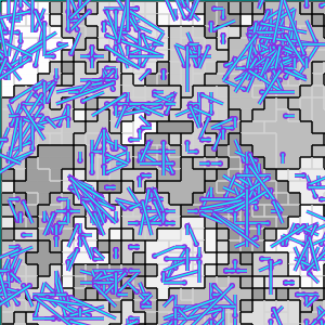
Figure B32CS:
Batch 32 case study overview.
Figures B32CS(b) through B32CS(e) are generated from a snapshot of a wild-type strain monoculture population.
In these images, each grid tile represents an individual cell.
Cells are organized into kin groups, color-coded by hue in Figure B32CS(b).
Established interconnects are overlaid in blue on Figure B32CS(c).
In Figures B32CS(d) and B32CS(e), kin groups are outlined in black.
Figure B32CS(d) highlights cells that are sending resource over-interconnect.
Figure B32CS(e) highlights cells that are receiving resource overinterconnect.
You can view an animation of the wild-type monoculture at https://mmore500.com/hopto/an.
This case study was drawn from epoch 18 of batch 32 from a secondary set of 64 evolutionary runs. These runs were identical to the first, except:
- increasing the default outgoing connection cap,
- making cells default-accept instead of default-reject intracellular messages from same-channel cells, and
- removing system-mediated parent-kin-group recognition to promote kin group turnover.
We set this strain aside for case study after preliminary screening suggested that over-interconnect messaging played an adaptive role and that the intercellular nature of the messaging was necessary to that adaptation.
The evolutionary history preceding this case study consumed approximately 72 hours of wall-clock time and 576 compute-core hours.
Approximately 2,197,976 simulation updates and 8,884 cellular generations elapsed.
You can view this case study strain in a live in-browser simulation at https://mmore500.com/hopto/7.
As before, we began by testing whether over-interconnect interaction was adaptive because of its intercellularity. We performed a competition experiment between the wild-type strain and a variant where over-interconnect messages were re-routed back to the sender. [Footnote TWAIR] The wild-type strain was present in greater abundance at the end of all 16 competitions (one-tailed binomial test; \(p < 0.0001\); 2/16 variant strain extinctions; 52 S.D. 3 cell gens elapsed). So the adaptiveness of over-interconnect messaging does depend on the intercellular nature of that messaging in this strain.
We proceeded to tease apart the evolved cellular mechanisms this messaging interacts with. We monitored hardware execution of the wild-type strain in a monoculture population to detect which signals, messages, and fork/call instructions activated each SignalGP module. %shorten because we already said it % put in common things into case study introduction Referring to a human-readable printout of the strain’s evolved genetic programming, we pieced together the hypothesized mechanism shown in Figure B32CS. It appears that neighboring a direct cellular offspring stimulates dispatch of an over-interconnect message that induces the recipient to pause somatic reproduction.
Four-hour competition experiments between wild type and knockout strains allowed us to assess the adaptiveness of each component of this mechanism.
We replaced the instruction responsible for over-interconnect messaging with a no-op instruction and observed a corresponding fitness penalty (16/16 knockout strain extinctions; one-tailed binomial test; \(p < 0.0001\); 416 S.D. 58 cell gens elapsed; https://mmore500.com/hopto/aa).
We also replaced the reproduction-pausing instruction executed in response to over-interconnect messaging with a no-op.
This caused a similar fitness penalty (16/16 knockout strain extinctions; 401 S.D. 29 cell gens elapsed).
To double-check whether messaging specifically over interconnects was key to adaptivity we also competed the wild-type strain against variants with the focal over-interconnect messaging instruction substituted for all other possible module-activating instructions:
- call (378 S.D. 42 cell gens elapsed;
https://mmore500.com/hopto/ac) - fork (377 S.D. 37 cell gens elapsed;
https://mmore500.com/hopto/ad) - internal message send (406 S.D. 39 cell gens elapsed;
https://mmore500.com/hopto/ae) - internal message send-to-all (422 S.D. 30 cell gens elapsed;
https://mmore500.com/hopto/af) - external message send (377 S.D. 37 cell gens elapsed;
https://mmore500.com/hopto/ag) - external message send-to-all (440 S.D. 32 cell gens elapsed;
https://mmore500.com/hopto/ah)
In each case the substitution variant strain was driven to extinction across all 16 replicate experiments (one-tailed binomial test; \(p < 0.0001\)).
The directionality of messaging over the interconnect, however, does not appear to affect fitness.
We tried substituting the wild-type instruction, which dispatches a message from the terminus of an interconnect to its origin, with an instruction that instead dispatches a message from the origin of an interconnect to its terminus.
In competition against wild-type, the wild type strain was more abundant in only ten of 16 replicate competitions (one-tailed binomial test; \(p = 0.2272\); 14/16 coalesced to a single strain; 410 S.D. 50 cell gen; https://mmore500.com/hopto/ai).
Next we assessed the adaptiveness of the particular spatio-temporal pattern of stimulation induced by incoming over-interconnect messages. Does this pattern differ from spatially and temporally random stimulation? If it does, is the non-uniformity of stimulation adaptive? To assess these questions, we measured the fraction of cells expressing module 14 in a monoculture wild-type population. Then, we created a variant strain where outgoing over-interconnect messages from module 5 were disabled and, instead, module 14 activated randomly with probability based on the empirical wild-type activation rate. [Footnote BOIBM]
In effect, this manipulation decouples reproductive pause from the distribution of over-interconnect message delivery and instead couples it to a comparable uniform random distribution. Indeed, in competition experiments against the wild-type strain this variant fares poorly (15/16 wild-type strain prevalent; 0 variant strain extinctions; one-tailed binomial test; \(p < 0.001\); 36 S.D. 2 cell gens elapsed), suggesting that the pattern of stimulation induced by over-interconnect messaging is meaningfully non-uniform. We confirmed this result with a larger-scale set of competition trials (58/64 wild-type strain prevalent; 0 strain extinctions; one-tailed binomial test; \(p < 0.0001\); 33 S.D. 2 cell gens elapsed).
Does the adaptively non-uniform pattern of stimulation induced by over-interconnect messages depend on non-uniform dispatch of messages from sending cells? To assess this question, we measured the per-cell frequency of module 5 activation in a monoculture wild-type population. We then created a variant strain where outgoing over-interconnect messages from module 5 were disabled. Instead, the over-interconnect message instruction was randomly executed with uniform per-cell probability based on the empirical wild-type execution rate. This variant strain held its own against the wild-type strain (5/16 wild-type strain prevalent; 0 strain extinctions; one-tailed binomial test; \(p = 0.9\); 30 S.D 1 cell gens elapsed). So, this strain’s non-uniform pattern of stimulation seems likely to result from the actual pattern of cell-cell interconnection rather than selective message dispatch.
We did not find evidence that cells were using tag-based developmental attractors or repulsors to bias connectivity (5/16 wild-type strain prevalent; 0 strain extinctions; \(p=0.9\); 35 S.D. 8 cell gens elapsed). However, we did notice frequent interconnect turnover via execution of both remove-incoming and remove-outgoing interconnect instructions. Substituting these instructions for no-ops yielded a knockout strain with lower fitness than wild-type (13/16 wild-type strain prevalent; 0 strain extinctions; one-tailed binomial test; \(p < 0.05\); 30 S.D. 11 cell gens elapsed). We confirmed this result with a larger-scale set of competition trials (60/64 wild-type strain prevalent; 0 strain extinctions; one-tailed binomial test; \(p < 0.0001\); 39 S.D. 5 cell gens elapsed). Is this remodeling of connectivity adaptively non-uniform? We measured the interconnect removal rate in a monoculture wild-type population. Then, we created a variant strain where interconnect-removal instructions were disabled. Instead, interconnects in this strain were removed randomly with uniform probability. In head-to-head competitions, this variant strain did not exhibit diminished fitness (20/64 wild-type strain prevalent; 0 strain extinctions; one-tailed binomial test; \(p = 1.0\); 30 S.D. 2 cell gens elapsed).
The adaptive mechanism of over-interconnect messaging at play in this strain remains somewhat unclear. Over-interconnect messaging induces an adaptively non-uniform pattern of module 14 activation. The transmission of messages between cells over the interconnects, in particular, contributes to fitness. When messages that would be delivered over interconnects are instead re-routed to the sending cell, fitness decreases. Substituting over-interconnect messaging for local messaging also decreases fitness. However, message dispatch is effectively random. This strain employs an adaptive during-lifetime interconnect-remodeling scheme. However, this remodeling scheme is also effectively random.
Although the process of interconnect development and retention might contribute some sort of spatial and/or temporal bias to module 14 activation, a full characterization of the nature of this bias and the mechanism inducing it remains elusive.
🔗 Wiring a Generic Small World Graph
Consider a set of computational nodes arranged in an \(r\)-dimensional mesh. In each dimension, physical interconnects run between immediately adjacent pairs of nodes. Represent this physical hardware with a graph \(N\). Vertices of \(N\), \(V(N)\), represent computational nodes. Edges of \(N\), \(E(N)\), represent physical interconnects between nodes.
Let \(d(a,b)\) represent the typical number of physical interconnects traversed on a shortest path between a pair of arbitrary nodes \(a, b \in V(N)\). This is conceptually equivalent to Manhattan distance.
In the case of a one-dimensional sequence of nodes, for a pair of arbitrary nodes \(a,b \in V(N)\),
Consider next the case of a higher-dimensional grid topology, like a two-dimensional grid or a three-dimensional mesh. Because \(d\) is a Manhattan metric, the number of physical interconnects requiring traversal in each dimension on a shortest-path between two nodes is completely independent.
Arranging the set of nodes \(N\) in a \(r\)-dimensional cube, cube width in each dimensions scales proportionally to the \(r\)-th root of \(|V(N)|\).
So, for a pair of arbitrary nodes \(a,b \in V(N)\),
We proceed to construct a small world directed graph \(G\) using the set of nodes \(N\) as vertices. In formal terms, a bijective relationship \(f: V(N) \rightarrow V(G)\) unites these two sets. The inverse mapping, \(f^{-1}: V(G) \rightarrow V(N)\), is also bijective.
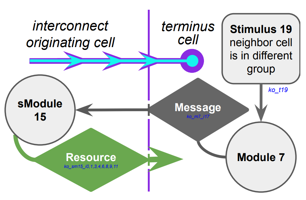
Edges in the graph \(G\) do not represent a physical interconnect. Instead, edges \(\{\hat{a}, \hat{b}\} \in E(G)\) represent a close-coordination relationship where node \(\hat{a}\) frequently interacts with (i.e., dispatches messages to) the destination node \(\hat{b}\). Figure RBACM illustrates the relationship between \(N\) and \(G\).
Let \(\hat{d}(\hat{a},\hat{b})\) denote distance between vertices \(\hat{a}\) and \(\hat{b}\) with respect to the graph \(G\). That is, the number of graph edges traversed on a shortest-path route between \(\hat{a}\) and \(\hat{b}\) over \(G\). In a small-world network, typical graph distance scales proportionally with the logarithm of network size [Watts and Strogatz, 1998]. In our case, for arbitrary \(\hat{a},\hat{b} \in V(G)\),
Consider the sequence of edges in \(G\) traversed on a shortest-path route \(R_{\hat{a},\hat{b}}\) between \(\hat{a}, \hat{b} \in V(G)\), \(\{\{\hat{v}_1, \hat{v}_2\}, \{\hat{v}_2, \hat{v}_3\}, \ldots, \{\hat{v}_{n-1}, \hat{v}_n\} \}\). If we traverse these same nodes over the graph \(N\) this path would be at least as long as the direct path between \(f^{-1}(\hat{a})\) and \(f^{-1}(\hat{b})\) over \(N\). (Otherwise, we would violate the Manhattan metric on \(N\)’s triangle inequality.) Therefore,
Recall that \(\hat{a},\hat{b}\) are sampled uniformly from \(V(G)\). So, \(f^{-1}(\hat{a}),f^{-1}(\hat{b})\) are sampled uniformly from \(V(N)\). Thus, Equation \ref{eqn:mesh_prop} allows us to establish the following lower bound,
It follows from Inequality \ref{eqn:path_hops_inequality} that
Equation \ref{eqn:smallworld_prop} tells us that the mean number of edges in \(R_{\hat{a}, \hat{b}}\) is proportional to \(\log(|V(G)|)\). So, letting \(\bar{d}\) represent the mean case,
Rearranging and simplifying, we arrive at a lower bound of mean distance over the Manhattan network \(N\) traversed for a connection in the interaction network \(G\),
Note that edges \(\{\hat{x},\hat{y}\}\) are not sampled uniformly from \(E(G)\). Instead, their sampling is weighted by edge betweenness centrality. [Footnote CAPON]
🔗 Wiring an Ideal Space-Filling Hierarchical Tree without Log-Time Physical Interconnects
Consider, again, a set of computational nodes arranged in an \(r\)-dimensional mesh. In each dimension, physical interconnects run between immediately adjacent pairs of nodes. Let this physical hardware corresponds to a graph \(N\) where \(V(N)\) represents computational nodes and \(E(N)\) represents physical interconnects between nodes.
Let \(d(a,b)\) represent the typical number of physical interconnects traversed on a shortest path between a pair of arbitrary nodes \(a, b \in V(N)\). This is conceptually equivalent to Manhattan distance.
Suppose we have a small-world graph \(G\) with maximum vertex degree bounded by a finite constant \(m\). The vertices of this graph \(G\) are embedded one-to-one on \(N\) such that \(|V(G)| = |V(N)|\). (Again, along the lines of Figure RBACM.)
Pick an arbitrary vertex \(a \in V(G)\). By the definition of a small-world graph,
Because the degree of the graph \(G\) is bounded by \(m\), there must be a subset \(T \subseteq G\) that, for some branching factor \(k \geq 2\) forms a complete \(k\)-nary tree rooted at \(a\) such that
- the tree height of \(T\) is \(h \propto \log |V(G)|\) and
- \(|V(T)| \propto |V(G)|\).
Legenstein and Maass establish a lower bound for the length of wiring required to construct a \(k\)-nary tree with \(n\) nodes on a one-dimensional \(L_1\) grid,
In our case, this corresponds to the total number of hops over \(N\) to traverse every edge in \(T\). Because, \(T \subseteq G\), \(\Omega(n \log n)\) is also a best-case lower bound for the total number of hops over \(N\) to traverse every edge in \(G\).
Because the degree of vertices in \(V(T)\) is bounded by \(k\),
In fact, because the degree of vertices in \(V(G)\) is also bounded by \(m\),
Let the wiring cost of an edge \(\{x, y\}\) in \(E(G)\) refer to the number of hops over \(N\) required to travel from \(x\) to \(y\). The best-case average wiring cost per edge can be computed as the best-case total wiring cost divided by the worst-case number of edges. For arbitrary \(\{x, y\} \in E(G)\),
This result applies to all possible small-world graphs \(G\) embedded on a one-dimensional computational mesh.
To tractably extend our analysis to three-dimensional meshes, rather than all small-world graphs we will specifically analyze the wiring cost of ideal space-filling trees [Kuffner and LaValle, 2009]. This construction efficiently distributes elements of \(G\) over \(N\) with respect to wiring cost. Although this construction potentially represents a lower bound on wiring cost, its optimality has not been concretely established.
For three dimensions, the total length of wiring required as a function of the number of nodes is
Because
we have \(w_3(n) \in \Theta \Big( n \Big)\). For an \(n\)-node tree, edge count \(|E(G)| \in \Theta \Big( |V(G)| \Big)\). So, average edge wiring cost remains constant as \(|V(G)|\) scales. Similar analysis concludes an equivalent result in the two-dimensional case.
🔗 Wiring an Ideal Space-Filling Hierarchical Tree with Log-Time Physical Interconnects
Once more, we will work with a mesh of \(n\) physical hardware nodes corresponding to a graph \(N\) where \(V(N)\) represents computational nodes and \(E(N)\) represents physical interconnects between nodes. In this case, in addition to physical interconnects between spatially adjacent nodes we will assume a system of hierarchical physical interconnects that allows log-hop traversal between nodes.
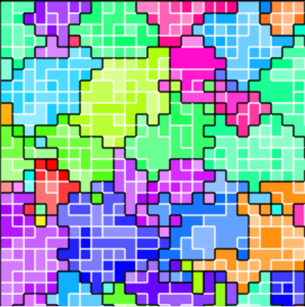
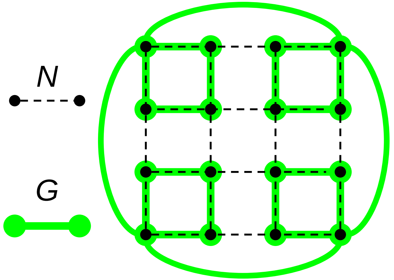 Figure ECOAI:
Example construction of an ideal space-filling tree over a computational mesh.
Figure ECOAI:
Example construction of an ideal space-filling tree over a computational mesh.
Suppose we have a small-world graph \(G\) with maximum vertex degree bounded by a finite constant \(m\). The vertices of this graph \(G\) are embedded one-to-one on \(N\) such that \(|V(G)| = |V(N)|\). We will specifically construct this graph as an ideal space-filling tree. Figure RBACM illustrates the relationship between \(N\) and \(G\).
As a property of this construction, \(|E(N)| \propto |V(N)|\).
In the best case, where edges in \(E(G)\) happen to correspond exactly to hierarchical physical interconnects \(E(N)\), the average hops required per edge is 1. However, in the worst case the average number of hops over \(N\) required per edge in \(E(G)\) is bounded by \(\log_m n\).
What if, instead of routing all traffic through log-time hierarchical interconnects, we routed traffic between nodes less than \(\log_m n\) apart through local grid-mesh interconnects?
In this case, we can bound worst-case total wiring cost by
For the space-filling tree on a one-dimensional mesh, we have \(m = 2\). Our upper bound on total wiring cost simplifies to
Because
we have \(w_2(n) \in \Theta \Big( n \times \log_2 \log_2 n \Big)\). Because edge count \(|E(G)| \in \Theta \Big( n \Big)\) we can establish the following upper bound on \(\bar{W}(n)\) mean wiring cost per edge in \(|E(G)|\) for the one-dimensional case,
What about the three-dimensional case? For the space-filling tree on a three-dimensional mesh, we have \(m = 8\). Our upper bound on total wiring cost simplifies to
Because
we have \(w_8 \in \Theta \Big( n \Big)\). Once more, because edge count \(|E(G)| \in \Theta \Big( n \Big)\) we can establish the following upper bound on \(\bar{W}(n)\) mean wiring cost per edge for the three-dimensional case,
🔗 Wiring a Watts-Strogatz Graph
Consider a set of computational nodes arranged in an \(r\)-dimensional mesh. In each dimension, physical interconnects run between immediately adjacent pairs of nodes. Represent this physical hardware with a graph \(N\). Vertices of \(N\), \(V(N)\), represent computational nodes. Edges of \(N\), \(E(N)\), represent physical interconnects between nodes.
Let \(d(a,b)\) represent the typical number of physical interconnects traversed on a shortest path between a pair of arbitrary nodes \(a, b \in V(N)\). This is conceptually equivalent to Manhattan distance.
In the case of a one-dimensional sequence of nodes, for a pair of arbitrary nodes \(a,b \in V(N)\),
Consider next the case of a higher-dimensional grid topology, like a two-dimensional grid or a three-dimensional mesh. Because \(d\) is a Manhattan metric, the number of physical interconnects requiring traversal in each dimension on a shortest-path between two nodes is completely independent.
Arranging the set of nodes \(N\) in a \(r\)-dimensional cube, cube width in each dimensions scales proportionally to the \(r\)-th root of \(|V(N)|\).
So, for a pair of arbitrary nodes \(a,b \in V(N)\),
We proceed to construct a small world directed graph \(G\) using the set of nodes \(N\) as vertices. In formal terms, a bijective relationship \(f: V(N) \rightarrow V(G)\) unites these two sets. The inverse mapping, \(f^{-1}: V(G) \rightarrow V(N)\), is also bijective.
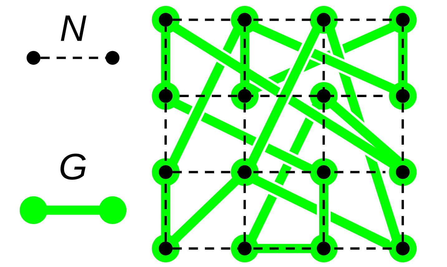 Figure RBACM:
Relationship between a computational mesh \(N\) and a small-world interaction network \(G\) constructed over \(N\).
Figure RBACM:
Relationship between a computational mesh \(N\) and a small-world interaction network \(G\) constructed over \(N\).
Edges in the graph \(G\) do not represent a physical interconnect. Instead, edges \(\{\hat{a}, \hat{b}\} \in E(G)\) represent a close-coordination relationship where node \(\hat{a}\) frequently interacts with (i.e., dispatches messages to) the destination node \(\hat{b}\). Figure RBACM illustrates the relationship between \(N\) and \(G\).
Let \(\hat{d}(\hat{a},\hat{b})\) denote distance between vertices \(\hat{a}\) and \(\hat{b}\) with respect to the graph \(G\). That is, the number of graph edges traversed on a shortest-path route between \(\hat{a}\) and \(\hat{b}\) over \(G\). In a small-world network, typical graph distance scales proportionally with the logarithm of network size [Watts and Strogatz, 1998]. In our case, for arbitrary \(\hat{a},\hat{b} \in V(G)\),
Suppose we have a small-world graph \(G\) constructed over a mesh \(N\) (as in Figure RBACM) using the Watts–Strogatz algorithm. In this procedure, vertices in \(V(G)\) corresponding to neighboring computational nodes in \(V(N)\) are wired together to form a lattice with mean degree \(k\). Then, for every vertex \(v \in V(G)\), each edge \(\{x, y\} \in E(G)\) containing \(v\) is reconfigured with probability \(0 < \beta < 1\) to connect \(v\) to a randomly-chosen node \(w \in V(G)\).
Before reconfiguration, the total wiring cost of \(G\) with respect to hops over \(N\) was proportional to \(|V(G)|\).
Recall that, with mesh dimensionality \(r\) we know that for a pair of arbitrary nodes \(a,b \in V(N)\),
So, after rewiring, the total wiring cost \(w\) of \(G\) with respect to hops over \(N\) can be calculated as
So, \(w \in \Omega \Big( |V(N)|^{\frac{r+1}{r}} \times r \Big)\).
In this graph, the number of edges is proportional to the graph size \(n\).
With bounded mean degree, we have \(|E(G)| \propto |V(G)|\) so we can establish the following lower bound on mean wiring cost per edge of \(G\) with respect to hops over \(N\),
Note that, with the introduction of log-time hierarchical hardware interconnects into \(N\) the mean wiring cost per edge of \(G\) with respect to hops over \(N\) is bounded in the worst case by \(\Omega \Big( \log |V(G)| \Big)\).
🔗 Conclusion
Ackley’s concept of indefinite scalability lays out an ambitious vision for the computational substrate of future open-ended evolution models. This vision has inspired researchers to incorporate thinking about underlying computational substrates into open-ended evolution theory and to consider how (or whether) available computational resources meaningfully constrain existing open-ended evolution models. For the time being, computational substrates for open-ended evolution limited purely by physical (or economic) concerns remain on the horizon, but indefinite scalability has already had concrete, and fruitful, impact on thinking around open-ended evolution.
Although prevalent contemporary computational hardware (and the developer-facing software infrastructure that supports its use) lacks essential features necessary to achieve true indefinite scalability such as fault tolerance and purely relative addressing, many cores are designed to support low-latency interconnects. These high-performance computing resources are increasingly accessible. Concern over indefinite scalability should not dissuade the design and implementation of open-ended evolution models that accommodate for the limitations of existing hardware and software infrastructure to make effective use of it. We highlight how log-time hardware interconnects might be exploited in practically scalable systems, but other model design or implementation tradeoffs may be relevant too (e.g., model dynamics or performance gains that rely on absolute instead of purely relative addressing).
Realizing open-ended evolution models with truly vast computational substrates will require intermediate steps. Efforts to pursue practical scalability that wrings out contemporary, commercially-available hardware and software infrastructure, will accelerate progress toward realizing truly indefinitely scalable systems. It seems conceivable that, coupled with innovative model design informed by open-ended evolution theory and effective model implementation in code, contemporary hardware systems and software infrastructure harbor the potential to realize paradigm-shifting advances in open-ended evolution. As was the case with deep learning, the tipping point of scale for model systems to exhibit qualitatively different behavior may be closer than we assume, perhaps only two or three orders of magnitude.
We highlighted how dynamic interactions within and between evolutionary individuals are crucial to open-ended evolution. Open-ended evolution models designed to scale computationally should realize these dynamic interactions within a framework that can be efficiently and readily mapped onto parallel computational implementation. Software tools that enable artificial life researchers to rapidly (and reusably) develop artificial life models have yielded substantial benefit to the field [Bohm and Hintze, 2017; Ofria et al., 2019]. Software tools or frameworks for parallel and distributed artificial life models that are versatile enough to support diverse use cases might help make practical scalability more practical. In particular, tools to collect data on distributed evolving systems (especially systematics tracking) seem likely to benefit the community.
Here, we presented an extension of the DISHTINY framework as an example of an artificial life system that might hypothetically take advantage of log-time hardware interconnects. We employed a very modest prototype parallel implementation that used shared-memory parallelism to distribute evolving — and interacting — populations of cells over two threads. We provided a faculty for cells to establish long-distance interconnects over the computational mesh, which in future implementations could rely on hardware-level log-time interconnects. We have characterized two strains that adaptively employed these interconnects to synthesize spatially-distributed functionality. In the first case study, messaging and resource sharing over interconnects appeared to facilitate resource recruitment to multicell peripheries. In a second case study, interconnect messaging played an adaptive role in selectively moderating somatic reproduction.
Incorporating simulation-level objects or physics in open-ended evolution models that explicitly correspond to hardware interconnects represents just one possible approach to exploiting them. Automatic detection of emergent long-distance interactions across a computational mesh and dynamically re-routing signaling traffic to use hierarchical interconnects might also be possible. Open-ended evolution models could also be entirely designed around hierarchical interconnects instead of a space-filling computational mesh.
At the core, from both the practical and indefinite standpoints, efforts to scale computational models of open-ended evolution seek to realize the evolutionary generation of continually novel and increasingly complex artifacts. As we scale DISHTINY, we are interested in assembling metrics to quantify different aspects of complexity in the system such as organization [Goldsby et al., 2012], structure, and function [Goldsby et al., 2014]. We believe that open-ended model systems built on contemporary distributed computational substrates will prove fruitful tools to investigate questions about how biological complexity relates to fitness, genetic drift over elapsed evolutionary time, mutational load, genetic recombination (sex and horizontal gene transfer), ecology, historical contingency, and key innovations.
🔗 Let’s Chat
I would love to hear your thoughts on scaling artificial life simulations and studying major transitions in evolution!!
I started a twitter thread (right below) so we can chat ![]()
![]()
![]()
nothing to see here, just a placeholder tweet 🐦
— Matthew A Moreno (@MorenoMatthewA) October 21, 2018
Pop on there and drop me a line ![]() or make a comment
or make a comment ![]()
🔗 Cite This Post
APA
Moreno, M. A., & Ofria, C. (2020, June 25). Practical Steps Toward Indefinite Scalability: In Pursuit of Robust Computational Substrates for Open-Ended Evolution. https://doi.org/10.17605/OSF.IO/53VGH
MLA
Moreno, Matthew A, and Charles Ofria. “Practical Steps Toward Indefinite Scalability: In Pursuit of Robust Computational Substrates for Open-Ended Evolution.” OSF, 25 June 2020. Web.
Chicago
Moreno, Matthew A, and Charles Ofria. 2020. “Practical Steps Toward Indefinite Scalability: In Pursuit of Robust Computational Substrates for Open-Ended Evolution.” OSF. June 25. doi:10.17605/OSF.IO/53VGH.
BibTeX
@misc{Moreno-Ofria-2020,
  title={Practical Steps Toward Indefinite Scalability: In Pursuit of Robust Computational Substrates for Open-Ended Evolution},
  url={osf.io/53vgh},
  DOI={10.17605/OSF.IO/53VGH},
  publisher={OSF},
  author={Moreno, Matthew A and Ofria, Charles},
  year={2020},
  month={Jun}
}
🔗 Footnotes
Footnote WDWCM Why do we consider mean node-to-node hops per connection?
Although relativistic concerns do ultimately limit latency between spatially-distributed computational elements, with respect to contemporary hardware co-located at a single physical site at foreseeable scales, we expect node-to-node hops to represent an important bottleneck on system performance.
At larger scales, consider the case where emergent connections are embodied via simulation state along the entire path of node-to-node hops traversed by the connection (along the line of axon wiring of biological neural networks). If mean emergent connections per simulation element remain constant as the system scales, then mean node-to-node hops per connection relates to the amount of state required per node to represent connections that pass through it. (Specifically, if mean node-to-node hops per connection remains constant then the amount of state required per node remains constant.)
Finally, the asymptotic analyses performed on mesh networks without long-distance hierarchical interconnects can be interpreted in terms of Euclidean distance. (Potentially of interest with respect to relativistic limitations.)
Footnote BOIBM Because over-interconnect broadcast messages activate all hardware units of a cell, we selected entire cells randomly and activated module 14 on all hardware units.
Footnote TWAOI This was an independent replication of the initial experiment (performed as part of a wider screen) that singled out the case study strain for further analysis.
Footnote CAPON Consider all pairings of nodes in a graph. Now, construct a multiset of paths that, for each possible node pairing, contains the shortest path between those two nodes. Edge betweenness is the fraction of the paths in this multiset that passes through a particular edge [Lu and Zhang, 2013].
🔗 References
Ackley, D. H. and Cannon, D. C. (2011). Pursue robust indefinite scalability. In HotOS.
Eiben, A. and Smith, J. E. (2015). Introduction to evolutionary computing. Springer, Berlin.
Gilbert, D. (2015). Artificial intelligence is here to help you pick the right shoes.
Lehman, J. (2012). Evolution through the search for novelty.
Markov, I. L. (2014). Limits on fundamental limits to computation. Nature, 512(7513):147–154.
🔗 Acknowledgements
Thanks to members of the DEVOLAB, in particular Santiago Rodgriguez-Papa for help developing the DISHTINY web interface. Thanks also to Ryan Moreno for feedback and suggestions on the asymptotic scaling proofs. This research was supported in part by NSF grants DEB-1655715 and DBI-0939454, and by Michigan State University through the computational resources provided by the Institute for Cyber-Enabled Research. This material is based upon work supported by the National Science Foundation Graduate Research Fellowship under Grant No. DGE-1424871. Any opinions, findings, and conclusions or recommendations expressed in this material are those of the author(s) and do not necessarily reflect the views of the National Science Foundation.