Evaluating Function Dispatch Methods in SignalGP
contents
🔗 Introduction
This work arises from collaboration with fellow-DEVOLAB student Alex Lalejini, whose research includes development of a new event-driven genetic programming system called SignalGP. His work aims to enable practitioners to better evolve agents that exhibit responsiveness to their surroundings — changing conditions in their environment & messages from other agents.
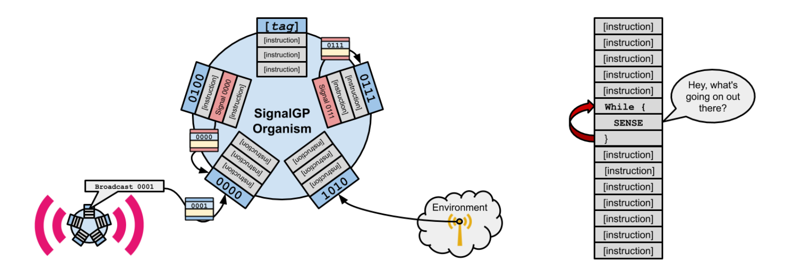 The stock SignalGP schematic (left) versus traditional linear genetic programming (right).
Courtesy Alexander Lalejini.
The stock SignalGP schematic (left) versus traditional linear genetic programming (right).
Courtesy Alexander Lalejini.
The idea is to organize instruction into tagged program sub-components and provide signal-dispatch infrastructure that accepts messages from other agents, environmental cues, and internally-generated signals (thread forks, function calls, etc.) and then boots up relevant program sub-component(s) in response.
(If you’re interested in more/better info here check out Alex’s super SignalGP blog post or [Lalejini & Ofria, 2018].)
The original implementation of SignalGP uses bitstring tags to match signals with responses. It takes a bitstring query, computes the query’s hamming distance (i.e., fraction aligned 0’s and 1’s) to all subcomponents’ tags, and then dispatches a single best match if half or more of that match’s tag’s 0’s and 1’s are aligned with the query. This particular method was chosen early on because it worked and was straightforward.
Pretty much since rubber hit the road with SignalGP, Alex has patiently entertained incessant queries and wild speculation from talk audiences (& especially from yours truly) on myriad alternate signal dispatch schemes.
- What if we use different types of tags besides bitstrings?
- What if we use different tag-matching metrics?
- What if match(es) were returned based on a match distance cutoff?
- What if tags were returned probabilistically based on match quality?
- What if tag-matching could be adjusted (e.g., “regulated”) at runtime?
These questions have been prominent on the SignalGP road map since the very beginning, so this summer we set out to make it happen. I had been interested in using tag-matching for other ends, so we decided to build an abstracted tag-matching tool that could be plugged in to SignalGP.
The tool is composed of three swappable modules,
- Metric: generates a raw match distance for each query/tag pair,
- Regulator: performs runtime adjustment of a tag’s match distances (e.g., a tag might be upregulated so that across the board it enjoys higher match distances or downregulated so that across the board it suffers lower match distances), and
- Selector: returns a subset of tags based on regulated match distances.
(If you use C++ and want to match some tags, the MatchBin class is available as a tool in our lab’s Empirical software library.)
In this work we explore the implications of two components of the MatchBin trifecta: Regulation and Selection. We’re investigating the implications of Metrics in other separate work.
Sometimes to get engineering things to work you have to try different things to see which one works best. This work is to some extent an exercise in fine tuning. But, if you stick around, there’ll also be some interesting evolutionary contingency, a cool (challenging?) distributed systems benchmarking problem, and some speculation on how evolved solutions are actually functioning.
🔗 Methods
This is the part where we chit-chat about the specifics of what we compared and how we compared them.
🔗 Benchmarking Problem
The primary design requirement behind our choice of diagnostic problem was that SignalGP instances would need to clue in to both the qualitative content and quantitative volume of exchanged messages. Our diagnostic problem is loosely inspired by quorum-sensing and collective decision-making tasks natural systems undertake [Miller & Bassler, 2001; Pratt et. al., 2002]. It also exhibits similarities to leader-election consensus problems SignalGP has been benchmarked on before, too [Lalejini & Ofria, 2018].
We arrange nodes in a toroidal (wraparound) grid where each cell interfaces with four neighbors. Each node is occupied by an independently-executing SignalGP instance. However, during evaluation all instances are loaded with the same SignalGP program.
There are two possible global underlying states and each node has a sensor. The task is for all cells to report the global underlying state.
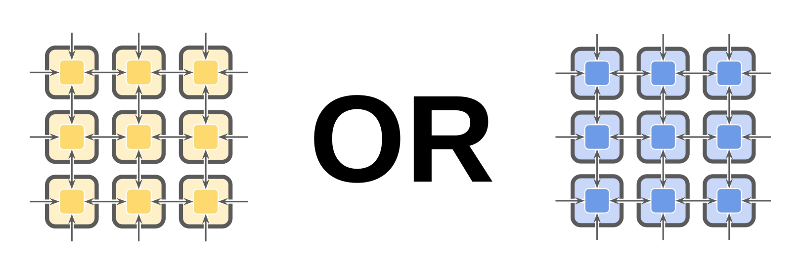 All nodes with reliable sensors.
In the schematic above, global underlying state is depicted by nodes’ lighter background color and sensor state is depicted by nodes’ darker foreground color. When all sensors correctly report global underlying state, the problem is trivial: the agent at each node can just output the reading of its own sensor.
However, when we introduce the possibility of faulty sensors, the problem becomes more difficult.
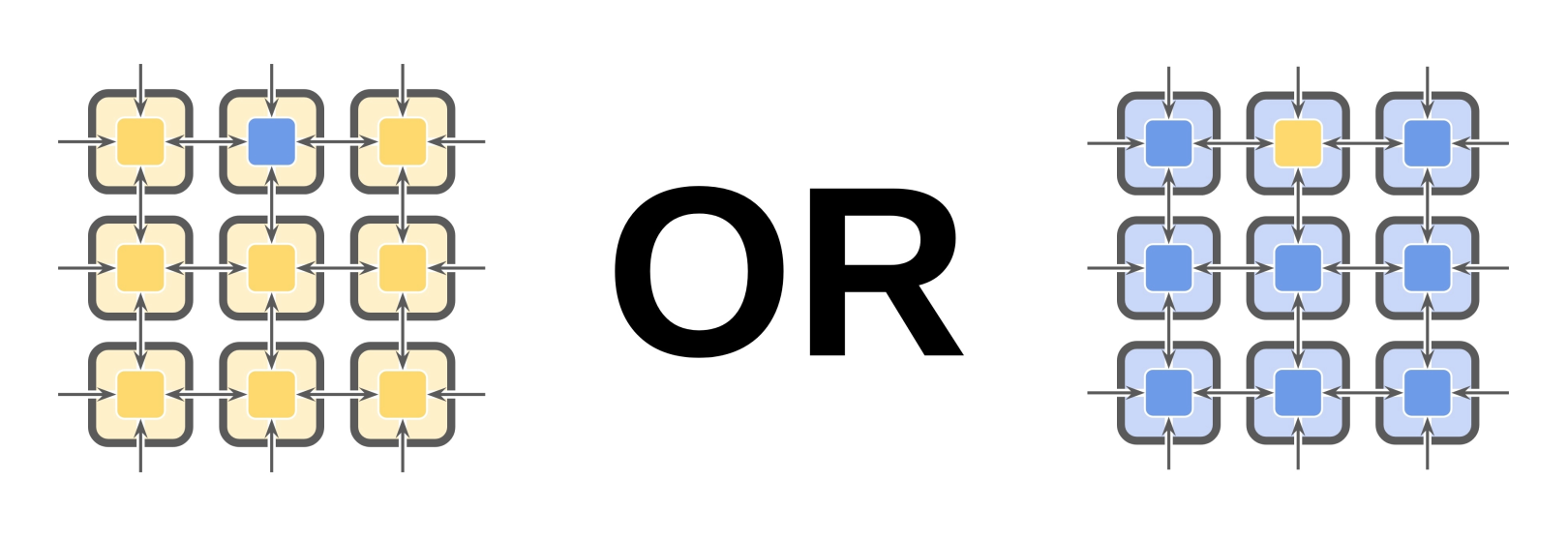 Eight nodes with reliable sensors, one with a faulty sensor.
In this example, the upper-center node exhibits a faulty sensor. When the underlying state is yellow, it reads blue. When the underlying state is blue, it reads yellow. The global state detection problem is still solvable, but now requires communication between nodes. (Agents at each node must check, and potentially adjust, their observation of global state based on observations reported by neighboring nodes.)
In subsequent diagrams, we will denote reliable sensors as green and faulty sensors as red. Faulty sensors always report incorrect state information.

 Comparison of reliable and faulty sensors.
We can adjust problem difficulty by changing the number of faulty sensors present in the group.
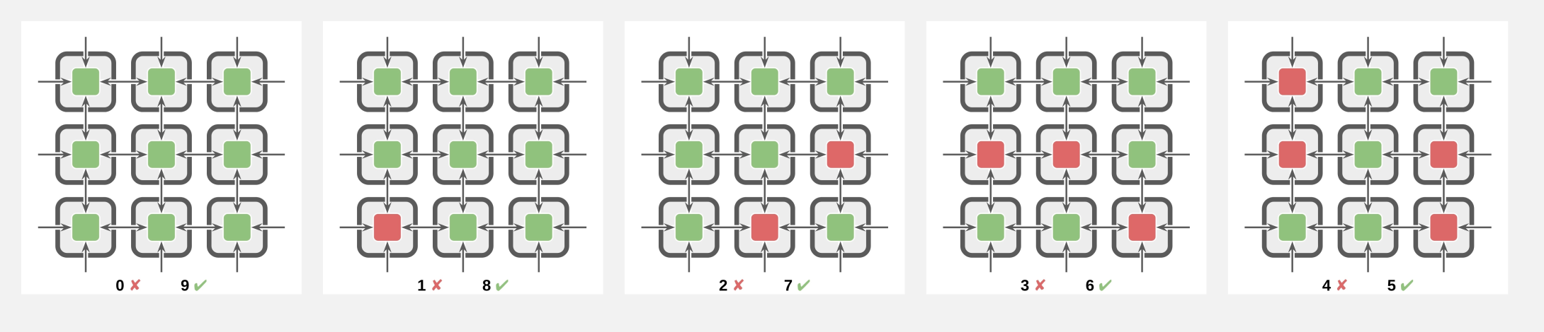 Problem difficulty varying from zero faulty sensors to nearly half faulty sensors.
Each problem difficulty level always has the same number of faulty sensors present in the group, but their arrangement is randomized at each evaluation.
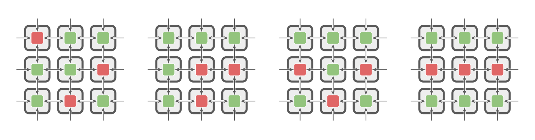 Randomized arrangement of faulty and reliable sensors.
We supplemented the standard SignalGP instruction set with experiment-specific instructions. These include,
-
Broadcast Message: insert a message into all four neighbors’ inboxes.
-
Send Message: insert a message into a random neighbor’s inbox.
-
Guess State: register the current node’s guess of underlying state. This guess is mutable and can be changed any time before the evaluation period ends.
-
Sense State: write the node’s state sensor reading into a memory register.
- Sensor state is also provided as an intermittent event-driven cue.
-
Random Number Generator: write a random number drawn uniformly from between 0 and 1 into a memory register.
- Individual nodes have no unique identifer — i.e., they’re nameless — but random number generators between nodes are decoupled, meaning this instruction could potentially be used to break symmetry between nodes.
Queued messages were delivered every eight hardware steps. Each evaluation afforded sixteen message exchange time-points.
If none of that clicked with you, try this bad D&D analogy on for size.
You come to in a dimly lit dungeon cell with no memory of who you are or how you got there. Your task is to figure out whether it’s daytime or nighttime. You can read your wrist watch, but it might not be set properly.
Every half hour the warden comes by to pick up and deliver messages. You can write any number of messages and choose to have them delivered to all four of your neighbors or to a random neighbor. Messages aren’t addressed, so you can’t tell which of your neighbors sent messages you receive.
Adventurers in the other cells are undertaking the same task and will use the same decision-making and communication strategies as you. You can only escape if all of you agree on the correct answer.
Roll a d6 for initiative.
🔗 Regulators
Tag-match regulation allows the SignalGP program module that will be returned by a particular query to be switched up at run time. A SignalGP program module can be “upregulated,” meaning that it will match better with every query against it. A program module can also be “downregulated,” meaning that it will match worse with every query against it. If a module is neither upregulated nor downregulated, its raw match distance with queries is unaffected.
Each tag designating a SignalGP program module has an associated regulation state. In this work, we use an unbounded floating point value. Negative values cause upregulation, positive values cause downregulation, and zero is neutral.
We provide the following instructions to interface with program modules’ regulation states,
- Set Regulator: set a module’s regulation state to a target value.
- Adjust Regulator: set a module’s regulation state from its current value a fraction towards a target regulation value.
- Sense Regulator: read a module’s current regulation state into a memory register.
Variants of each instruction determine which program module to interface with by an unregulated query-lookup and by the currently-executing program module (e.g., self).
After a set number of decay cycles designated when a regulation value is set or adjusted, we automatically decay regulation state to neutral. We provide an instruction, Extend Regulator, that performs an unregulated query-lookup then pads the decay countdown of that program module’s regulation value.
In this work, we compare a control no-operation regulation module with two functional regulation variants.
- additive regulator: adjust raw match distance by a fixed amount, with the result clamped between 0.0 and 1.0.
return std::clamp( std::tanh(regulation_state) + raw_distance, 0.0, 1.0 ); - multiplicative regulator: adjust raw match distance a fixed fraction towards 0.0 (upregulated) or 1.0 (downregulated).
return raw_distance + std::tanh(state) * ( state < 0 ? raw_distance : 1.0 - raw_distance ); - no-op regulator: perform no adjustments to raw match distance.
return raw_distance;
The following figure compares these three regulation methods.
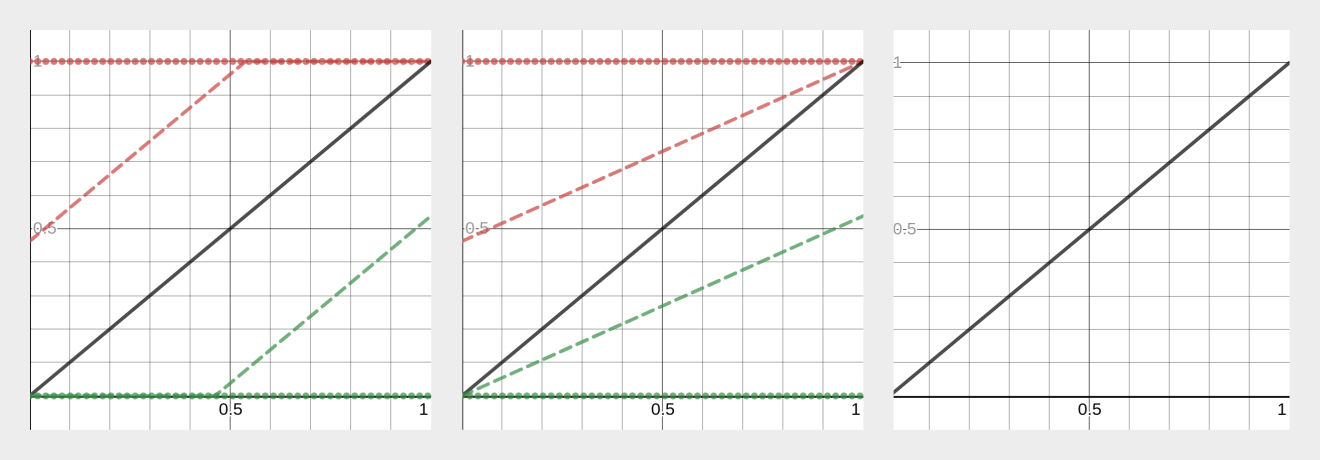 Additive (left), multiplicative (center), and no-op (right) regulators.
In this depiction, x represents raw match distance and y represents regulated match distance.
Dashed red lines are weakly downregulated and dotted red lines are strongly downregulated.
Dashed green lines are weakly upregulated and dotted green lines are strongly upregulated.
Additive (left), multiplicative (center), and no-op (right) regulators.
In this depiction, x represents raw match distance and y represents regulated match distance.
Dashed red lines are weakly downregulated and dotted red lines are strongly downregulated.
Dashed green lines are weakly upregulated and dotted green lines are strongly upregulated.
🔗 Selectors
Selectors receive the match distances of tagged SignalGP program components with respect to the current query and determine which program component is returned.
In this work, we compare three selectors,
- depo selector: if a query matches with a program component beyond a cutoff threshold, increase the component’s cumulative activation score based on match quality and an extra “query strength” runtime parameter; return all program components with cumulative activations that surpass a threshold and set the components’ cumulative activation to a negative (suppressed) starting-point. Intermittently decay all cumulative activation scores back to zero.
- ranked selector: sort all program components by match distance and return the best-matching program component if it surpasses a cutoff threshold.
- sieve selector: return all program components with match distances that surpass a cutoff threshold.
The depo (“depolarization”) selector is the odd one out here. Unlike other selectors, which are stateless query-to-query, the depo selector’s behavior in response to a current query may be influenced by past queries. We devised it to mimic the dynamics of neural systems where a cellular response is triggered by the aggregate impact of multiple inputs.
The ranked and sieve selectors serve as controls for the depolarization selector. The ranked selector, which emulates the behavior of previous SignalGP work, only ever returns one result at a time. The sieve selector, like the depo selector, may potentially return more than one result at a time.
The following figure overviews schematics of these three selectors.
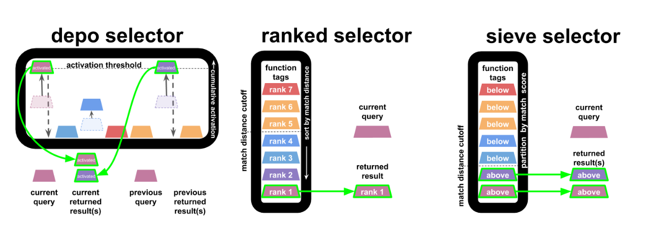 Schematic comparing selectors.
In all experiments, the ranked selector was used for function calls and regulation instruction lookups. Depending on the treatment, other selectors handled incoming messages, environmental cues, and function forks.
🔗 Experiments & Treatments
We evolved solutions on two grid sizes: a small 3 × 3 grid consisting of nine agents and a large 9 × 9 grid consisting of 81 agents.
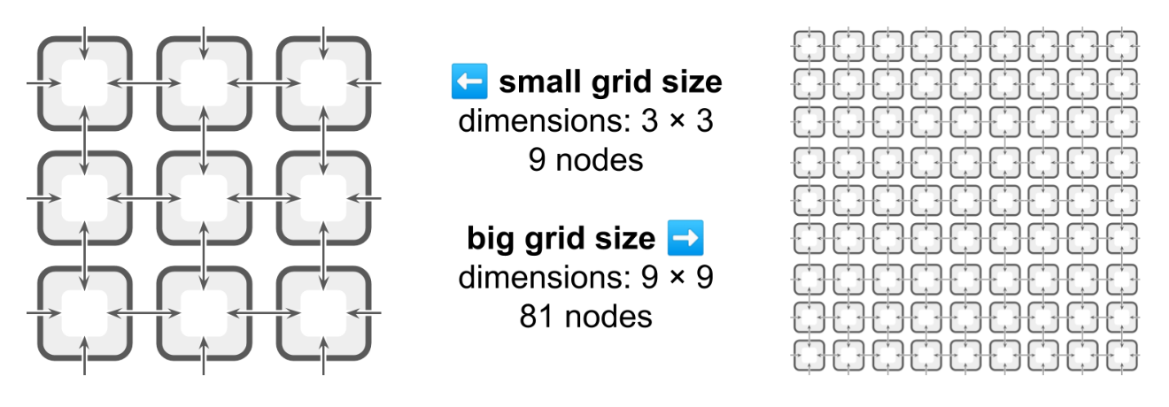 Small and large toroidal grid sizes.
We evolved solutions on five tiers of problem difficulty:
- 0% faulty (0/9 or 0/81 faulty),
- ~11% faulty (1/9 or 9/81 faulty),
- ~22% faulty (2/9 or 18/81 faulty),
- ~33% faulty (3/9 or 27/81 faulty), and
- ~44% faulty (4/9 or 36/81 faulty).
We worked with three regulator schemes:
- additive,
- multiplicative, and
- no-op.
We worked with three selector schemes:
- depo,
- ranked, and
- sieve.
We performed two experiments: one to assess the impact of regulators on evolved solutions and the other to assess the impact of selectors on evolved solutions. We will present results and discussion for each experiment separately.
In the first experiment, we assessed all combinations of the following conditions:
- grid size
- small
- problem difficulty
- ~11% faulty
- ~44% faulty
- regulator
- additive
- multiplicative
- no-op
- selector
- depo
- ranked
- sieve
- tag-matching metric
- streak [Downing, 2015; p. 226]
(The second experiment revealed qualitatively similar results evolving on small and large grid sizes and that ~11% and ~44% faulty problem difficulties exhibited qualitatively different evolutionary outcomes).
In the second experiment, we assessed all combinations of the following conditions:
- grid size
- small
- large
- problem difficulty
- ~0% faulty
- ~11% faulty
- ~22% faulty
- ~33% faulty
- ~44% faulty
- regulator
- multiplicative
- selector
- depo
- ranked
- sieve
- tag-matching metric
- streak [Downing, 2015; p. 226]
(The first experiment revealed that additive and multiplicative regulators both significantly outperformed the no-op regulator. Additive and multiplicative regulators exhibited similar performance with multiplicative regulation slightly, but not significantly, outperforming additive regulation.)
In both experiments, each treatment was evaluated in ten replicate runs.
🔗 Fitness & Selection
We calculated fitness as the fraction of agents that correctly guessed underlying global state. We supplemented fitness such that ties were broken by the fraction of agents that made any guess about underlying global state. Finally, any ties at this stage were broken by the fraction of agents that guessed differently than their sensor reading. Perfect fitness — all agents correctly guessing underlying global state — was capped at 1.0.
During evolution, we evaluated programs on their mean performance across two evaluations, one with each underlying global state. (Fitness trajectories over evolutionary time report these values.) At the end of evolutionary runs, we evaluated programs on their mean performance across 200 evaluations, 100 with each underlying global state. (Final solution qualities report these values.) At the end of evolutionary runs, we also evaluated solutions on the grid-size opposite that they evolved on (solutions that evolved on small grids evaluated on a large grid and vice versa). Here, fitness was also calculated as mean performance across 200 evaluations, 100 with each underlying global state.
We evolved unstructured populations of 100 individuals. We employed tournament selection with tournament size two. (We chose to evolve with weak selection pressure to slow selective sweeps.) Programs were propagated asexually using standard SignalGP mutation parameters without elitism or crossover.
🔗 Code, Data, Statistics, and Computation
Source code to replicate our experiments and analyses are available on GitHub. Data and figures are available via the Open Science Framework.
We performed exploratory runs to generate testable hypotheses then performed a second set of runs with different random number generator seeds to evaluate our hypotheses. All figures, statistical results, and archived raw data are drawn from the second set of runs.
We ran our computational experiments on Michigan State University’s High Performance Computing Center. Small grid (3 × 3) evolutionary runs completed 2500 generations in several minutes up to around four hours. Large grid (9 × 9) evolutionary runs completed 1000 generations in around an hour up to around twelve hours.
🔗 Results & Discussion: Regulators
We found that at the 44% faulty problem difficulty tier, the no-op regulator significantly underperformed both the additive and multiplicative regulators in terms of mean solution quality and perfect solution discovery frequency. In fact, the only perfect solutions discovered at this problem difficulty tier employed the additive and multiplicative regulators. No perfect solutions evolved at this tier with the no-op regulator.
We did not discern a difference in performance between the additive and multiplicative regulators or a difference in performance between any regulators at the 11% faulty problem difficulty tier.
🔗 Mean Solution Quality
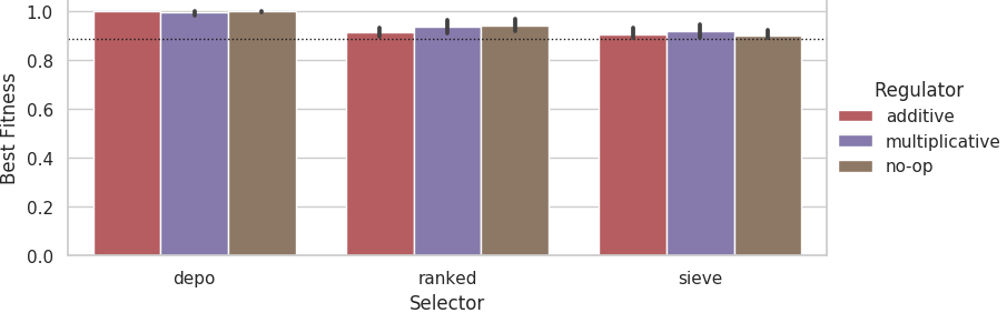 Mean best fitness at the end of evolutionary runs on the 11% faulty problem difficulty tier across 10 replicates.
Dashed lines indicate fitness score that could be achieved if each agent outputted its own sensor value.
Error bars represent 95% confidence intervals.
Mean best fitness at the end of evolutionary runs on the 11% faulty problem difficulty tier across 10 replicates.
Dashed lines indicate fitness score that could be achieved if each agent outputted its own sensor value.
Error bars represent 95% confidence intervals.
At 11% difficulty tier, with the depo selector all regulators achieve near-perfect fitness across trials. With the ranked and sieve selectors, all regulators perform worse but still comparably.
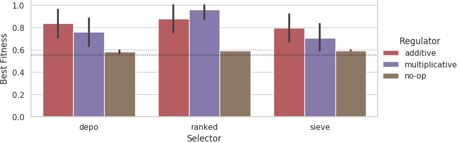 Mean best fitness at the end of evolutionary runs on the 44% faulty problem difficulty tier across 10 replicates.
Dashed lines indicate fitness score that could be achieved if each agent outputted its own sensor value.
Error bars represent 95% confidence intervals.
Mean best fitness at the end of evolutionary runs on the 44% faulty problem difficulty tier across 10 replicates.
Dashed lines indicate fitness score that could be achieved if each agent outputted its own sensor value.
Error bars represent 95% confidence intervals.
At the 44% difficulty tier, the no-op regulator significantly under-performs the additive and multiplicative regulators (non-overlapping 95% CI). The additive and multiplicative regulators appear to perform comparably.
🔗 Perfect Solution Frequencies
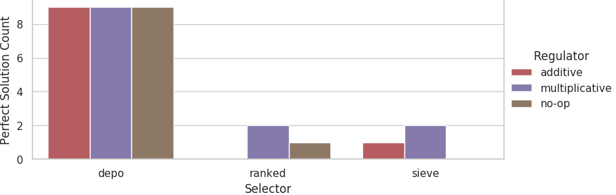 Counts of evolutionary runs at the 11% problem difficulty tier that evolved perfect solutions out of 10 replicates.
At the 11% problem difficulty tier, equivalent counts of perfect solutions evolved for each regulator with the depo selector. We did not detect a significant difference in the rates that perfect solutions evolved between the no-op and additive/multiplicative regulators for the ranked and sieve selectors.
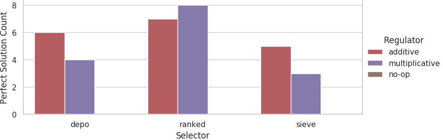 Counts of evolutionary runs at the 44% problem difficulty tier that evolved perfect solutions out of 10 replicates.
At the 44% problem difficulty tier, the no-op selector evolved no perfect solutions. The additive regulator evolved significantly more perfect solutions than the no-op selector across all three selectors (Fisher’s exact tests; 6/4 vs 0/10, p = 0.011; 7/3 vs 0/10, p = 0.003; 5/5 vs 0/10, p = 0.0325). The multiplicative regulator evolved significantly more perfect solutions with the ranked selector than the no-op regulator. We did not detect a significant difference in the rates that perfect solutions evolved between the no-op and multiplicative regulators for the depo and sieve selectors.
🔗 Results & Discussion: Selectors
We found that, on low-tier problem difficulties the depo selector significantly outperformed the ranked and sieve selectors in terms of mean solution quality and perfect solution discovery frequency.
In fact, among evolutionary runs on the big grid, we observed a significantly greater frequency of perfect solution discovery at higher-faulty problem difficulty tiers. This greater number of perfect solutions observed on the higher-faulty difficulty tiers might be due to contingency on an intermediate evolutionary state. Perhaps evolved solutions based on regulation may commonly arise via a precursor solution where an agent’s guess at global underlying state becomes decoupled from the reading of its onboard sensor but not yet effectively coupled to communication from neighboring agents. This intermediate state might be more strongly selected against in regimes where the agent’s onboard sensor tends to be more reliable.
The depo selector’s stronger performance on low-tier problem difficulty might then be interpreted in terms of circumventing this contingency by providing an alternate evolutionary pathway to incorporate messages from neighbors.
Indeed, we also found that, on these low-tier problem difficulties the depo selector evolved solutions that exhibited different outcomes when scaled from the small grid to the large grid and vice versa. Solutions evolved under these conditions which perform perfectly at one grid size are significantly more likely to fail to perform perfectly at the other grid size. This difference in scaling behavior further suggests that on low-tier problem difficulties solutions evolved with the depo selector rely on special mechanistic underpinnings.
This effect appeared more prominent among solutions evolved on the small grid size. The effect was present, but less pronounced, among solutions evolved on the big grid size.
The depo selector seems, therefore, to enable greater evolutionary flexibility but, because we found that it performed comparably to other selectors at the higher faulty problem difficulty tiers, not necessarily meaningful functionality that cannot also be achieved through the program module regulation system.
🔗 Mean Solution Quality
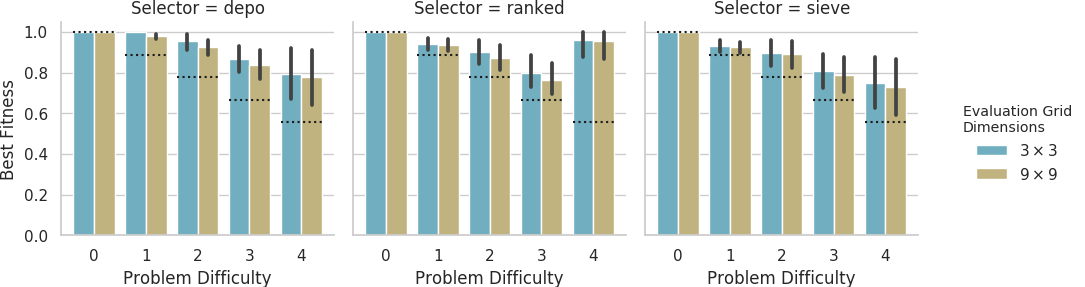
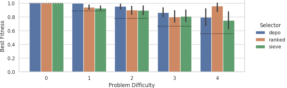 Mean best fitness at the end of evolutionary runs on the small grid size across 10 replicates.
Dashed lines indicate fitness score that could be achieved if each agent outputted its own sensor value.
Error bars represent 95% confidence intervals.
Mean best fitness at the end of evolutionary runs on the small grid size across 10 replicates.
Dashed lines indicate fitness score that could be achieved if each agent outputted its own sensor value.
Error bars represent 95% confidence intervals.
For the small grid size problem, the depo selector significantly outperformed the ranked and sieve selectors at the 11% problem difficulty tier (non-overlapping 95% CI).
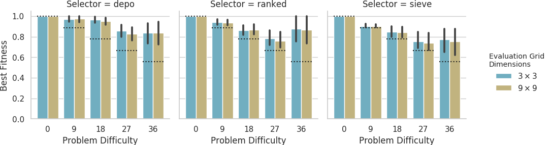
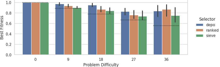 Mean best fitness at the end of evolutionary runs on the big grid size across 10 replicates.
Dashed lines indicate fitness score that could be achieved if each agent outputted its own sensor value.
Error bars represent 95% confidence intervals.
Mean best fitness at the end of evolutionary runs on the big grid size across 10 replicates.
Dashed lines indicate fitness score that could be achieved if each agent outputted its own sensor value.
Error bars represent 95% confidence intervals.
For the big grid size problem, the depo selector significantly outperformed the ranked and sieve selectors at the 22% problem difficulty tier (Kruskal-Wallis H-tests; h=3.90, p=0.048; h=4.97, p=0.026).
🔗 Perfect Solution Frequencies
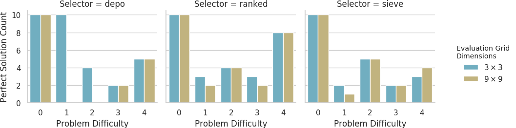
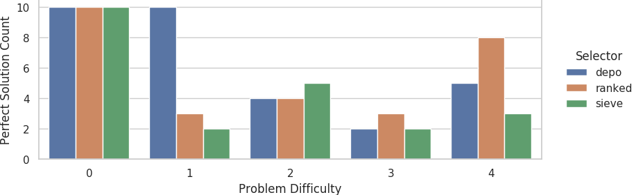 Counts of evolutionary runs on the small grid size that evolved perfect solutions out of 10 replicates.
On the small grid at the 11% faulty problem difficulty tier, the depo selector evolves perfect solutions at a significantly higher rate than both the ranked and sieve selectors (Fisher’s exact tests; 10/0 vs. 3/7, p=0.003; 10/0 vs. 2/8, p=0.0007).
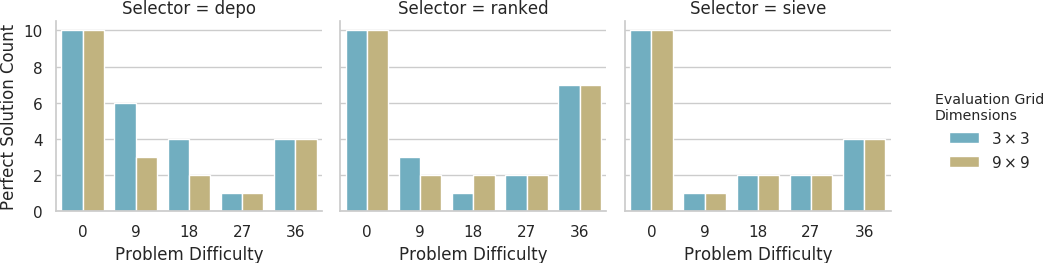
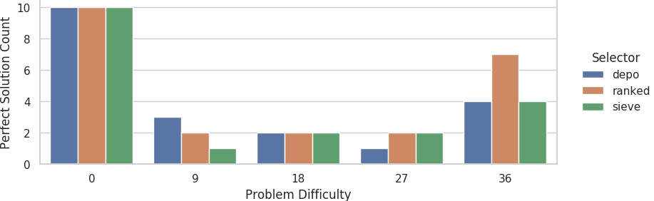 Counts of evolutionary runs on the large grid size that evolved perfect solutions out of 10 replicates.
Interestingly, for the big grid size, we observed significantly more perfect solutions at the 44% faulty problem difficulty tier than at the 22% faulty problem difficulty tier (Fisher’s exact test, 6/24 vs. 15/15, p=0.029).
We were not able to detect a significant difference in the rate that perfect solutions evolved between the 22% and 44% faulty difficulty tiers for the small grid size.
We can also see that significantly more perfect solutions evolve with the depo selector on the small grid at the 11% problem difficulty tier than on the large grid at that same problem difficulty tier (Fisher’s exact test, 10/0 vs. 3/7, p=0.0031). We’ll circle back around to this observation in the next section.
🔗 Solution Scalability
In order to assess the qualitative mechanisms underlying evolved solutions, we analyzed the behavior of solutions in the grid size opposite that they evolved in. (Solutions evolved on the small grid size were evaluated on the large grid size and solutions evolved on the large grid size were evaluated on the small grid size.)
The plots below compare counts of solutions that evaluated perfectly on the small grid and evaluated perfectly on the large grid. For the most part, solutions evaluated perfectly either on both grid sizes or perfectly on just one grid size. (Thus, members of the lower count category would all also rank as members of the higher count category.) We did detect, and account for in our analyses, one case to the contrary. Among solutions evolved on the big grid at the 22% problem difficulty tier with the depo selector, we found two perfect solutions when evaluated on the big grid size, four perfect solutions when evaluated on the small grid size, but only one solution that was evaluated perfectly on both grid sizes.
 Counts of evolutionary runs on the small grid size out of 10 replicates that evolved perfect solutions when evaluated on the small grid size and on the large grid size.
All perfect solutions evolved with the depo selector on the small grid size at problem difficulty tiers 1 and 2 did not yield perfect evaluations on the large grid size. However, all perfect solutions evolved with the depo selector at problem difficulty tiers 3 and 4 did yield perfect evaluations on the large grid size. Between these problem difficulty tiers, the rate of successful scaling to the large problem difficulty tiers did differ significantly (Fisher’s exact test, 14/0 vs. 0/7, p < 0.00001).
We also compared the counts of solutions that performed perfectly on both grid sizes and those that performed perfectly on just one grid size between the depo selector at problem difficulty tiers 1 and 2 and other selectors across all non-trivial problem difficulty tiers. The depo selector at problem difficulty tiers 1 and 2 had a significantly higher rate of solutions that performed perfectly on just one grid size than both the ranked selector (Fisher’s exact test, 14/0 vs. 2/16, p < 0.00001) and the sieve selector (Fisher’s exact test, 14/0 vs. 2/16, p < 0.00001).
 Counts of evolutionary runs on the large grid size out of 10 replicates that evolved perfect solutions when evaluated on the small grid size and on the large grid size.
Looking at solutions that evolved on the big grid, we also observed several solutions that performed perfectly on just one of the evaluation grid sizes at problem difficulty tiers 1 and 2. There was a significantly higher fraction of solutions that performed perfectly on just one grid size with the depo selector at problem difficulty tiers 1 and 2 compared to problem difficulty tiers 3 and 4 (Fisher’s exact test, 7/4 vs. 0/5, p=0.034).
🔗 Conclusion
The primary objective of this work was to evaluate the relative efficacies of regulator and selector components of the SignalGP function dispatch process.
We found that the solutions evolved with the additive and multiplicative regulator modules outperformed or matched the performance of the no-operation regulator module. Regulation functionality appeared critical to solving the 44% faulty sensor problem difficulty tier: we observed no perfect solutions evolve with the no-operation module. However, we did not discern a difference in the performance between the additive and multiplicative regulator modules.
We also found that the depo selector outperformed the ranked and sieve selectors at lower faulty-rate problem difficulty tiers. However, selectors performed comparably at higher faulty-rate problem difficulty tiers. We suspect that solutions evolved with the depo selector can exploit unique mechanisms to sidestep apparent evolutionary contingency at the lower faulty-rate problem difficulty tier. However, because solutions evolved with all selectors achieved comparable performance at higher faulty-rate problem difficulty tiers, we interpret our observations as evidence that the depo selector enables greater evolutionary flexibility but not necessarily meaningful functionality that cannot also be achieved through the program module regulation system.
Both of these results evidence the utility of plastic, during-lifetime adjustments to program module dispatch in SignalGP. This observation adds a subtle twist to insight about the future work of SignalGP.
Among other objectives, in proposed “Multi-representation SignalGP” work we aim to expand the set of computational representations underpinning SignalGP modules beyond linear genetic programs [Lalejini and Ofria, 2019]. Hintze et al. have demonstrated practical benefits of evolving digital agents composed of heterogeneous computational representations, which they refer to as the “Buffet Method” [Hintze et al., 2019]. In their work, agents’ connectivity between modules is genetically determined and immutable during an agent’s lifetime. The buffet paradigm allows evolving agents to rely on computational representations best-suited to a problem at hand, but also to hybridize representations to efficacious ends. With the addition of dynamic module dispatch via selector and regulator components, “Multi-representation SignalGP” promises not only to realize the benefits of the Buffet Method in interactive, event-driven agents but also provide a framework for module-level plasticity.
🔗 Cite This Post
🔗 APA
Moreno, M. A.(2019, December 16). Evaluating Function Dispatch Methods in SignalGP. https://doi.org/10.17605/OSF.IO/RMKCV
🔗 MLA
Moreno, Matthew A. Evaluating Function Dispatch Methods in SignalGP. OSF, 16 Dec. 2019, doi:10.17605/OSF.IO/RMKCV.
🔗 Chicago
Moreno, Matthew A. 2019. “Evaluating Function Dispatch Methods in SignalGP.” OSF. December 16. doi:10.17605/OSF.IO/RMKCV.
🔗 BibTeX
@misc{moreno2019evaluating,
  title={Evaluating Function Dispatch Methods in SignalGP},
  url={osf.io/rmkcv},
  DOI={10.17605/OSF.IO/RMKCV},
  publisher={OSF},
  author={Moreno, Matthew A},
  year={2019},
  month={Dec}
}
🔗 References
🔗 Acknowledgements
Thanks to members of the DEVOLAB, in particular Nathan Rizik for help implementing gene regulation features in SignalGP and Alexander Lalejini for his comments on my draft of this blog. This research was supported in part by NSF grants DEB-1655715 and DBI-0939454, and by Michigan State University through the computational resources provided by the Institute for Cyber-Enabled Research. This material is based upon work supported by the National Science Foundation Graduate Research Fellowship under Grant No. DGE-1424871. Any opinions, findings, and conclusions or recommendations expressed in this material are those of the author(s) and do not necessarily reflect the views of the National Science Foundation.
🔗 Let’s Chat!
Questions? Comments? Ideas on where we should take this work next? (Especially’d love to hear your ideas about applications!)
I started a twitter thread (right below) so we can chat ![]()
![]()
![]()
working w/ @amlalejini on program module regulation for #SignalGP & wrote up some first results showing how it helps evolve good solutions to a distributed sensing/consensus problem (explained w/ bad D&D analogy🤷♂️)https://t.co/T8gku0eQ1Y
— Matthew A Moreno (@MorenoMatthewA) December 17, 2019
excited where this work is headed next!
🔗 Supplementary Figures
🔗 Regulation Experiment
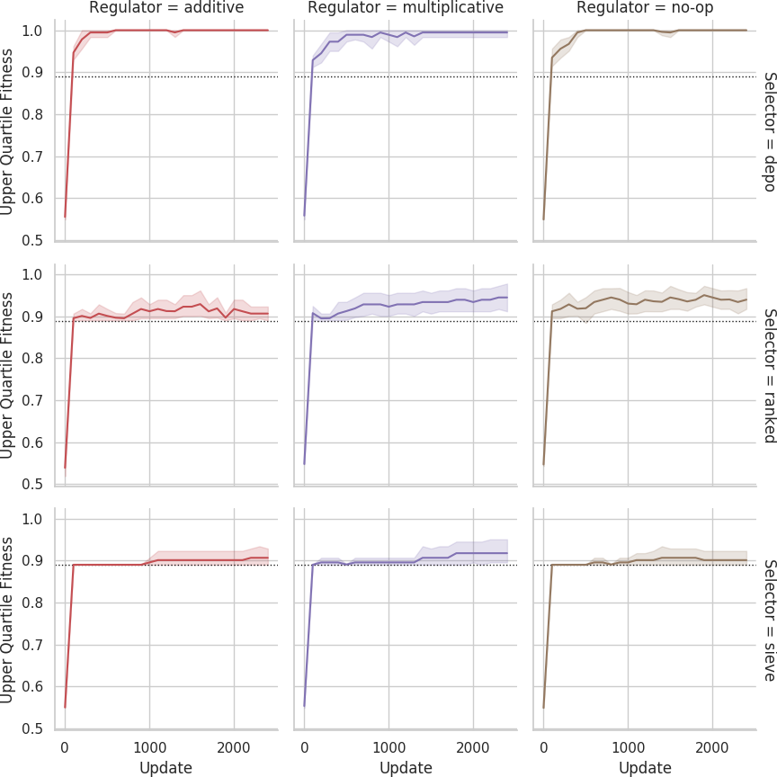 Mean fitness across replicates over evolutionary time for the 11% faulty problem difficulty tier.
Dashed lines indicate fitness score that could be achieved if each agent outputted its own sensor value.
Shaded bands are 95% confidence intervals.
Mean fitness across replicates over evolutionary time for the 11% faulty problem difficulty tier.
Dashed lines indicate fitness score that could be achieved if each agent outputted its own sensor value.
Shaded bands are 95% confidence intervals.
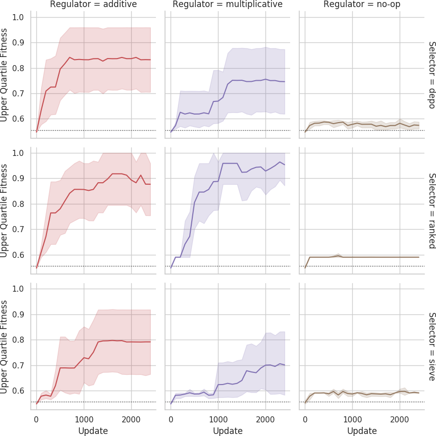 Mean fitness across replicates over evolutionary time for the 44% faulty problem difficulty tier.
Dashed lines indicate fitness score that could be achieved if each agent outputted its own sensor value.
Shaded bands are 95% confidence intervals.
Mean fitness across replicates over evolutionary time for the 44% faulty problem difficulty tier.
Dashed lines indicate fitness score that could be achieved if each agent outputted its own sensor value.
Shaded bands are 95% confidence intervals.
 Distribution of best fitness values for the 11% faulty problem difficulty tier.
Dashed line indicates fitness score that could be achieved if each agent outputted its own sensor value.
Distribution of best fitness values for the 11% faulty problem difficulty tier.
Dashed line indicates fitness score that could be achieved if each agent outputted its own sensor value.
 Distribution of best fitness values for the 44% faulty problem difficulty tier.
Dashed line indicates fitness score that could be achieved if each agent outputted its own sensor value.
Distribution of best fitness values for the 44% faulty problem difficulty tier.
Dashed line indicates fitness score that could be achieved if each agent outputted its own sensor value.
🔗 Selector Experiment
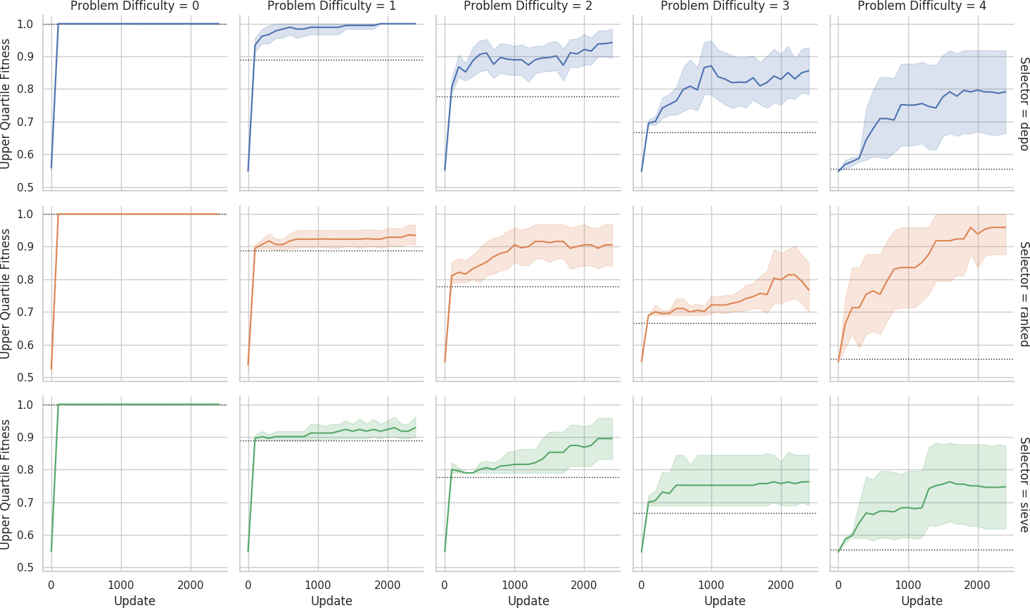 Mean fitness across replicates over evolutionary time on the small grid.
Dashed lines indicate fitness score that could be achieved if each agent outputted its own sensor value.
Shaded bands are 95% confidence intervals.
Mean fitness across replicates over evolutionary time on the small grid.
Dashed lines indicate fitness score that could be achieved if each agent outputted its own sensor value.
Shaded bands are 95% confidence intervals.
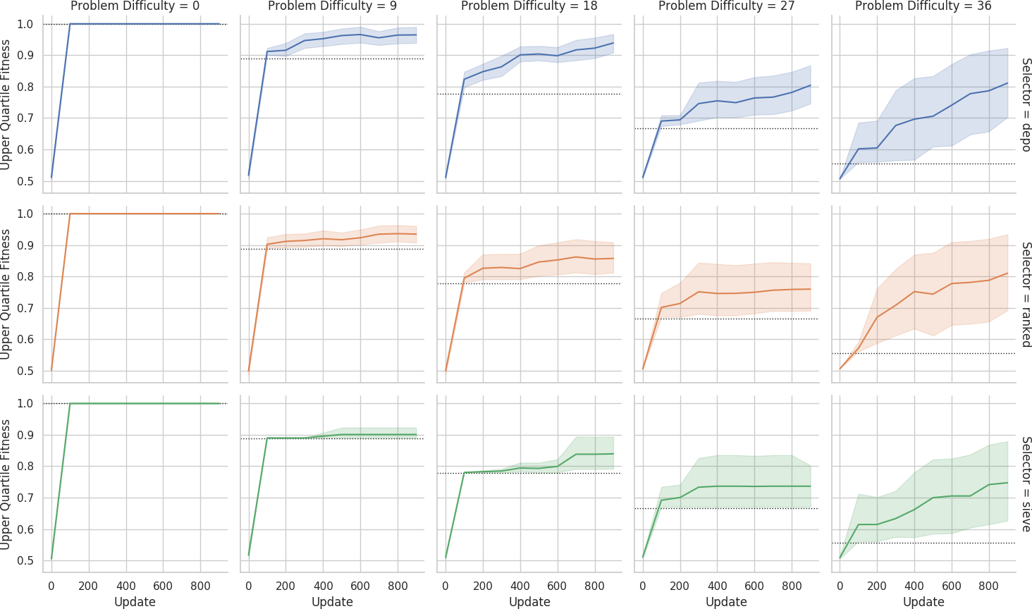 Mean fitness across replicates over evolutionary time on the big grid.
Dashed lines indicate fitness score that could be achieved if each agent outputted its own sensor value.
Shaded bands are 95% confidence intervals.
Mean fitness across replicates over evolutionary time on the big grid.
Dashed lines indicate fitness score that could be achieved if each agent outputted its own sensor value.
Shaded bands are 95% confidence intervals.
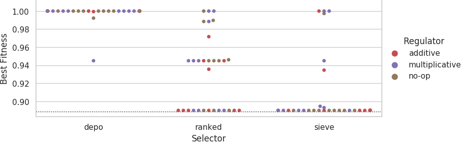
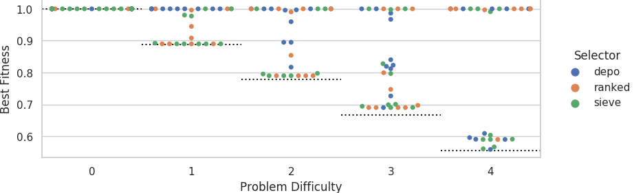 Distribution of best fitness values on the small grid.
Dashed lines indicate fitness score that could be achieved if each agent outputted its own sensor value.
Distribution of best fitness values on the small grid.
Dashed lines indicate fitness score that could be achieved if each agent outputted its own sensor value.
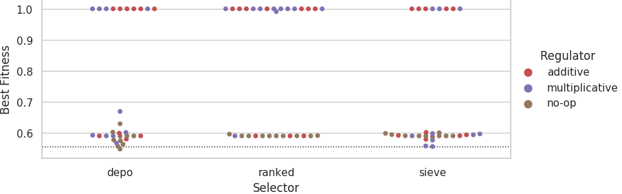
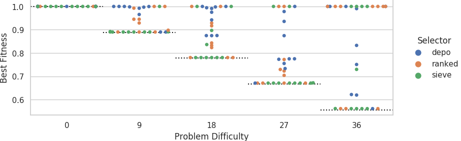 Distribution of best fitness values on the big grid.
Dashed lines indicate fitness score that could be achieved if each agent outputted its own sensor value.
Distribution of best fitness values on the big grid.
Dashed lines indicate fitness score that could be achieved if each agent outputted its own sensor value.
 Mean best performance of solutions evolved on the small grid evaluated on small and big grids.
Dashed lines indicate fitness score that could be achieved if each agent outputted its own sensor value.
Mean best performance of solutions evolved on the small grid evaluated on small and big grids.
Dashed lines indicate fitness score that could be achieved if each agent outputted its own sensor value.
 Mean best performance of solutions evolved on the big grid evaluated on small and big grids.
Dashed lines indicate fitness score that could be achieved if each agent outputted its own sensor value.
Mean best performance of solutions evolved on the big grid evaluated on small and big grids.
Dashed lines indicate fitness score that could be achieved if each agent outputted its own sensor value.